Cluster Rasch models for microarray gene expression data

(1)

comment

reviews

reports

deposited research

interactions

information

refereed research

Research

Cluster-Rasch models for microarray gene expression data

Hongzhe Li and Fangxin Hong

Address: Rowe Program in Human Genetics, Departments of Medicine and Statistics, University of California, Davis, CA 95616, USA.

Correspondence: Hongzhe Li. E-mail: hli@dna.ucdavis.edu

Abstract

Background: We propose two different formulations of the Rasch statistical models to the

problem of relating gene expression profiles to the phenotypes. One formulation allows us to investigate whether a cluster of genes with similar expression profiles is related to the observed phenotypes; this model can also be used for future prediction. The other formulation provides an alternative way of identifying genes that are over- or underexpressed from their expression levels in tissue or cell samples of a given tissue or cell type.

Results: We illustrate the methods on available datasets of a classification of acute leukemias and

of 60 cancer cell lines. For tumor classification, the results are comparable to those previously obtained. For the cancer cell lines dataset, we found four clusters of genes that are related to drug response for many of the 90 drugs that we considered. In addition, for each type of cell line, we identified genes that are over- or underexpressed relative to other genes.

Conclusions: The cluster-Rasch model provides a probabilistic model for describing gene expression

patterns across samples and can be used to relate gene expression profiles to phenotypes. Published: 31 July 2001

GenomeBiology2001, 2(8):research0031.1–0031.13

(Print ISSN 1465-6906; Online ISSN 1465-6914)

Received: 26 February 2001 Revised: 11 May 2001 Accepted: 19 June 2001

Background

Recently, DNA chip or microarray technology has been developed that allows researchers to measure the expression levels of thousands of genes simultaneously over different time points, different experimental conditions or different tissue samples. It is based on the hybridization of DNA or RNA molecules with a library of complementary strands fixed on a solid surface. Oligonucleotide chips contain thou-sands of features with gene-specific sequences about 25 bases long. These oligos are then hybridized with labeled probe derived from a given tissue or cell line. The resulting fluorescence intensity gives information about the abun-dance of the corresponding mRNA. This is the Affymetrix DNA chip technology. Alternatively, cDNA can be spotted on nylon filters or glass slides. Complex mRNA probes are reverse transcribed to cDNA and labeled with red or green fluorescent dyes. This technique is often called the spotted

array or cDNA array. In both methods, thousands of mRNA concentrations can be measured in parallel, potentially revealing complex gene regulatory networks.

(2)

drugs and, therefore, aid in the process of drug discovery and provide a rationale for selection of therapy on the basis of the molecular characteristics of a patients tumor.

From the statistical point of view, the challenge is that the microarray gene expression data are often measured with a great deal of noise, and that the sample size of tissues or cell lines, denoted by n, is usually very small compared to the number of genes in expression arrays, denoted by p. This results in the large p, small n problem [5]. Most current approaches to dealing with this problem first select genes that can best separate tissues of different types by performing uni-variate analysis. The expression levels of these genes are then combined linearly in a weighted way to form compound covariates. These covariates are then used in the standard regression models for model fitting and prediction. West et al. [5] proposed a Bayesian binary regression approach using the singular value decomposition to first reduce the dimen-sion of the variable space (p) to the number of samples (n). They called the resulting linear combination of the expression levels of all the genes the expression of the supergenes. All these approaches reduce the variable space by making one or several linear combinations of the expression levels of some or all of the genes. Linear combination may not, however, be the best way of reducing the dimension of the variable space.

Another popular approach to analyzing gene expression data is to use clustering methods to simultaneously cluster both samples and genes in order to determine some clusters of genes that are mostly correlated with some clusters of samples. Examples of such an application include analysis of gene expression data and drug response for the 60 human cancer cell lines of the National Cancer Institute (NCI60 data) [4], and analysis of cancerous and normal colon tissues [2]. However, the clustering approach is purely exploratory and requires an external similarity measure. Methods that can be used to assess the significance of the clustering results are needed.

The Rasch model (RM) and its extensions [6,7] are an impor-tant staple of psychological research and are used in other fields such as sociology, educational testing and medicine. The idea of the RM is that one can indirectly infer a persons position on a latent trait from his/her responses to a set of well-chosen items. For example, the RM has been used to infer the quality of life of cancer patients from their answers to a well-designed questionnaire [8], or to measure disability from activities of daily living [9]. For these applications, data are usually given in a matrix, with rows being individuals and columns being responses to a set of items. Microarray gene expression data are also given in a transposable matrix form with rows being genes and columns being samples, and vice versa. The RM can therefore be used to explain the observed patterns over different columns. Here we propose two different formulations of the polytomous RM for analy-sis of microarray gene expression data. The first formulation

treats samples as persons and genes as items. The idea is to infer several latent factors associated with a given sample on the basis of its expression profile over many genes. We combine a model-based clustering method [10] with the RM to define a small set of latent factors associated with samples. For a given sample, we assume that genes in the same cluster determine one latent factor associated with this sample, and use the RM to estimate this latent factor for each gene cluster. These latent factors are then used in a regression analysis of the observed phenotypes. The rational of this approach is that genes of similar function yield similar expression patterns in microarray hybridization experiments [11-13]. Co-regulated genes may share similar expression profiles, maybe involved in related functions or regulated by common regulatory elements [14]. Therefore, if genes are clustered together, it is impossible from a statisti-cal point of view to differentiate one gene from the other. In this case, a better way of studying these genes is to treat them as a cluster. Consideration of genes in the same cluster can potentially reduce noise associated with a single gene.

The second formulation is to treat genes as persons and samples as items. The idea is to infer several latent factors associated with each gene based on its expression levels across samples from different tissue or cell types. This formulation provides simple summary statistics for genes based on their expression profiles over samples, and helps to identify genes that are more likely be over- or underexpressed within samples of the same type or between samples of different types. We first briefly review some key ideas of the polytomous RM and its estimation. We then present two different formulations of the RM for the gene expression data. Details involved in these formulations are given. We apply our proposed methods to the analysis of the leukemia dataset [1] and the NCI60 dataset [4] and conclude with discussion of our method.

Results

The Rasch model (RM)

The RM was originally proposed as an item-response theory model in the psychological test or attitude scale [6]. The idea is that the use of a test or scale presupposes that one can indirectly infer a persons position on a latent trait from his/her responses to a set of well-chosen items. Assume that we have I persons and J items. Let Zijbe the response of individual ito the item j, where the response can take one from m + 1 possible ordinal categories, 0, , m. One version of the RM, which we use in this paper, called the partial credit model [15], assumes the probability of response h, as

PrZij= h=

exphai+bjh

, (1)

m

l=0 explai+bjl

(3)

comment

reviews

reports

interactions

information

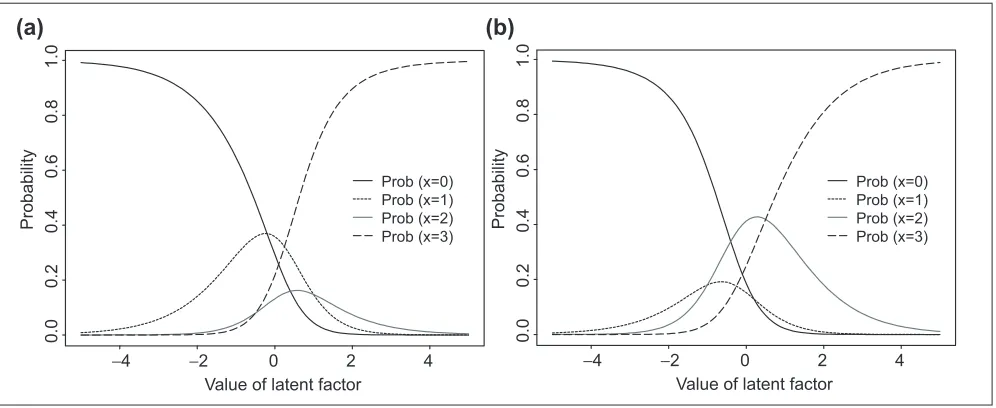
of the respective level lof item j. aiis the person parameter that expresses the latent factor of the ith person that is mea-sured by the Jitems. It is easy to verify that the probability of the response is monotonous in both person and item parameters. For example, for m= 3, Figure 1 plots the Rasch probabilities as a function of the value of the latent factor (a) for two sets of item-specific b values. It can be seen from these plots that for a given item, persons with larger avalue tend to have greater probability of expressing high scores, and for a given person, the response probabilities are differ-ent for items with differdiffer-ent bvalues. To make the model (1) identifiable, the following constraints are required

bjm=0, for j= 1, . . . , p, and

j

l

bjl=0

Therefore, there is a total of Jm- 1 unconstraint item-spe-cific parameters.

The item parameters can be estimated based on the condi-tional likelihood, given minimal sufficient statistics for the person parameters. For a given person, the minimal suffi-cient statistic is the sum of the category weights correspond-ing to the observed responses. After the b parameters are estimated, the person parameters can then be estimated by maximizing the likelihood function. Details on the condi-tional likelihood estimation of the item parameters can be found in Anderson [16].

Relating gene expression profiles to phenotypes Typical microarray data consist of expression levels for a large number of genes on a relatively small number of samples. Let xijbe the gene expression level of the jth gene in the ith sample, for i= 1, , n, and j= 1, ..., p. In practice,

n is usually much smaller than p. For spotted arrays, to moderate the influence of gene expression ratios above and below one, we may apply the natural log transform to all the red to green ratios [12]. Upregulated genes thus have a positive log expression ratio, whereas downregulated genes have a negative log expression ratio. Or xij might be the expression level from an oligonucleotide array. In addition, for the ith sample, we have observed phenotype yi, which could be a binary indicator such as two different types of cancer, a continuous measurement such as drug-response activity or censored survival time such as time to tumor recurrence. To apply the RM to the gene expression data xij, we first need to discretize the gene expression levels xij into zij, which takes value from 0, ..., m, for i= 1, ..., n, j= 1, ..., p. In practice, we can use the quantiles or the quantiles within quantiles as cut-off points for discretization. Because this approach uses only ranks rather than the actual expression levels, there may be slight loss of infor-mation. However, in return, we gain a valid analysis with robustness to the outliers.

Outline of the approach

[image:3.609.57.555.493.697.2]

Our goal is to infer several latent factors associated with each sample based on its gene expression profile, and relate these latent factors to the observed phenotypes. Using the terms of the RM, we treat each gene as an item, each tissue sample or cell line as a person, and treat the expression level as the response of a given tissue to a given gene. The unidimen-sional RM may not, however, hold for the complete set of genes generated by microarrays. Here we assume that genes with similar expressions determine one latent factor, and that the RM holds for each set of genes with similar expres-sion profiles.

Figure 1

Example of Rasch probabilities as a function of the value of the latent factor for an item with four different response categories for two different sets of item-specific parameters (a) b= (0.3,0.5,-0.5,0) and (b) b= (-0.3,-0.5,0.5,0).

Value of latent factor

Probability

−4 −2 0 2 4

0.0

0.2

0.4

0.6

0.8

1.0

Prob (x=0) Prob (x=1) Prob (x=2) Prob (x=3)

Value of latent factor

Probability

−4 −2 0 2 4

0.0

0.2

0.4

0.6

0.8

1.0

(4)

To identify genes with similar expression profiles over samples, we first use the model-based clustering method of Fraley and Raftery [10] to cluster pgenes into K clusters based on their gene expression profiles over nsamples. Note that the cluster-step is performed based on the observed continuous gene expression data, not the discretized gene expression patterns. For a given sample, using expression profiles of genes in a given cluster, we estimate a latent factor by fitting a RM. These latent factors are then used in a regression analysis to study the relationship between the gene expressions and the phenotype. The method allows to investigate whether a cluster of genes with similar expres-sion profiles is related to the observed phenotypes, and can also be used for future prediction by estimating the latent factors using the maximum likelihood estimation. We give some details for each of these steps in the following sections.

Model-based clustering analysis

Cluster analysis, based on multivariate normal mixture models [10,17], has been used for clustering various types of biological, zoological, financial and industrial data. We first set up the mixture model for the gene expression data. Let xj= {x1j, ...,xnj} be the n-dimensional vector of the jth gene expression over nsamples. We assume that the gene expres-sion values of pgenes, x1, ..., xp, arise from a mixture of K n-dimensional Gaussian distribution with density

f(X)= K

k=1tkfnXú mk,k, (2)

where the tkis the probability that a gene belongs to the kth cluster, and fn(X|mk,Sk) denotes the density function of the multivariate normal distribution with mean mkand variance-covariance matrix Sk. Possible parameterization of the covari-ance matrix is discussed in Fraley and Raftery [10]. Note that if we assume a simple covariance structure, Sk=lI, where Iis the identity matrix, and lis the variance, then the model-based clustering method becomes the K-means clustering method [18].

Treating clustering as a mixture model problem allows us to use the EM algorithm to estimate the probability of a given gene belonging to each of the Kclusters, and to estimate the corresponding mean vector and covariance matrix for each cluster [10]. One advantage of this approach is that it allows us to obtain an estimate of the number of gene clusters. Fol-lowing Fraley and Raftery [10], we propose to use the Bayesian inference criterion (BIC) [19] for selecting the number of gene clusters. BIC is defined as

BIC(K) = 2L(K) - nKlog p,

where L(K) is the maximized log-likelihood, nK is the number of independent parameters to be estimated in the K-cluster model and p is the sample size (number of the genes). We will choose K that gives the maximum BIC(K) value.

As the first step of our approach, we cluster genes into K clus-ters using the model-based clustering method described above, where the number of gene clusters Kis determined by maxi-mizing the BIC scores. Let Ckdenote the genes in cluster k, and pkdenote the number of genes in this cluster, for k= 1, ..., K.

Rasch model and regression analysis

We fit a RM model as in equation (1) for genes in each of the Kclusters respectively, treating samples as persons and genes as items. To fit the RM (equation 1) for genes in the kth cluster, we let ibe the sample index, and jbe the gene index, for i= 1, ..., n, and j= 1, ..., pk, and let ai= aikin model (1) be the latent factor for the ith sample which is determined by the genes in the kth cluster, and bjlbe the gene-specific parameter for the jth gene. The RM assumes that the variation of the gene expression patterns observed over different samples is due to a latent factor, and it provides a probabilistic model to describe the gene expression pattern for a given sample.

Let âik be the maximum likelihood estimate of the latent factor for the ith sample determined by the genes in the kth cluster. Let âi= (âi1, ...,âiK) be the vector of the estimated latent factors based on the gene expression profiles for the ith sample. In general, we can relate the phenotype yifor the ith sample to the estimated of latent factors âiby a regres-sion model,

yi=fa^i;g+ei, (3)

for i= 1, ..., n, where gis the vector of regression parameters,

eiis the error term, and the actual model of the regression function (f) and the distribution of the error depend on type of the phenotype. If the phenotype is a continuous variable, linear regression can be used, if it is a binary variable, logis-tic or probit regression can be used, and if the phenotype is survival time, the Cox regression model can be used. Alter-natively, the generalized linear model can be used. One advantage of the proposed method is that we can model the interactions between the latent factors in the standard way of modeling interactions in the regression models. As only the estimated and not the observed latent factors are avail-able in the regression model (equation 3), the variance of the estimate of the gparameter has to be corrected. We propose to use a two-step bootstrap resampling procedure [20] to estimate the variance of the estimate of the parameter gin the regression model. First, within the kth gene cluster, we resample genes and re-estimate the aikparameter by fitting the RM (1). Second, for a given set of estimated a parame-ters, we resample the nsamples from (yi,^ai), for i= 1, ..., n, and fit the regression model (equation 3) to obtain a new estimate of g. We can then estimate the variance of ^gwith these resampled estimates.

Prediction

(5)

according to the clustering result. For a gene jin cluster k, we first discretize its expression level into one of the m + 1 categories using the cut-off points used in the discretization-step, denoted by znew,j. We can then estimate the corre-sponding latent factor ak by maximizing the following likelihood function,

Lak=

⌸

jÎCk

PrZnew,j= znew,júak,b^jh, (4)

where ^bjhis the estimated gene-specific parameter for gene j in the kth cluster based on the training sample. Using the estimated vector of the latent factors ^a, the regression model (3) can then be used for predicting phenotype Ynew.

RM for latent factors associated with genes

The second formulation of the RM for gene expression data is to treat genes as persons, and samples as items. Assume that we have gene expression data of p different genes, indexed by i, over nksamples of the kth sample type, indexed by j, for k= 1, ..., K. Note that the indices iand jare used dif-ferently from the previous sections. We are interested in identifying genes that are expressed differently among these different sample types. Here each gene has its own expres-sion patterns over different samples. For gene i, we can esti-mate a latent factor aikbased on its gene expression profile over nksamples from the kth sample type by fitting the RM (equation 1), for k= 1, ..., K. In this formulation of the RM, we treat genes as persons, treat samples as items, and treat each genes expression level over samples as the responses. In RM (1), I= p, and J= nk, ai= aik, which is the latent factor for the ith gene determined by the samples of the kth type, and bjlis the sample-specific parameter. This model assumes that the variation of gene expression patterns across differ-ent samples among differdiffer-ent genes is due to several gene-specific latent factors. Here the latent factor aik can be interpreted as some quantities related to the transcription factors of the ith gene which determine the gene expression levels in samples of the kth sample type. For a given tissue or cell line type k, genes with larger estimated latent factor (aik) tend to have higher expression levels than those with smaller estimated latent factor. For a given sample type k, the esti-mated latent factors, (^a1k}, ..., ^apk), provide a nice way to order genes based on their expression levels over a small number of samples of sample type k, and to identify genes that are relatively over- or underexpressed in the kth sample type. In addition, by comparing the estimated latent factors associated with genes across different sample types, we can identify genes that are differentially expressed among differ-ent tissue or cell line types.

Analysis of the leukemia dataset Classification using cluster-RM

We applied the proposed approach to the problem of classify-ing acute leukemias. Acute leukemias can broadly be divided into two classes, acute myeloid leukemia (AML) and acute lymphoblastic leukemia (ALL), that originate, respectively,

from cells of myeloid or lymphoid origin. The two diseases appear identical under the microscope. However, correct diagnosis is critical, as they respond best to different treat-ment regimens. Golub et al. [1] used a set of 38 leukemia samples including 11 AML and 27 ALL as training samples set, and used an additional 34 samples (14 AML, 20 ALL) as a test set for testing their proposed method for class predic-tion. In our analysis, we combined both the training and the test datasets into a dataset of 72 samples (25 AML and 47 ALL). For each of the 72 samples, the gene expression data were extracted from Affymetrix expression arrays.

We first selected the subset of 3,571 genes based on an initial processing adopted by the authors of the leukemia study. The expressions summarized are the log (base 10) values of the actual expression levels following this initial filtering and transformation. We then select 50 genes that are mostly over-expressed in AML, and 50 genes that are mostly overover-expressed in ALL by using the Wilcoxon rank sums test. This simple rule of selecting a smaller set of genes are also used in Golubet al. [1] using slightly different tests. As expected, the model-based clustering method assuming the common covariance matrix clusters these 100 genes into two clusters, with 50 genes in each cluster. The left plot of Figure 2 shows the gene expres-sion levels of these 100 genes for the 72 leukemia samples. Clearly, these 100 genes are highly differentially expressed between the two types of the leukemia samples.

Given the 100 genes selected, methods such as principal component analysis, partial least-square regression or com-posite covariate predictor can be used to further reduce the gene dimension to two or three dimensions by taking linear combinations of the gene expression levels. Instead of taking linear combination of gene expression levels, we first dis-cretize the expression levels of all the 100 genes over 72 samples into four categories using the quantiles as the cut-off points. Therefore, for each gene, their expression level can take one of four possible values of 0, 1, 2 and 3. The same analysis was also done by discretizing gene expression levels into eight categories, the results were essentially the same. In the following, we only present the results using four categories. Fitting two RMs to these discretized gene expres-sion levels, we estimate two latent factors for each sample; one latent factor is determined by gene expression profiles of 50 genes in one cluster, the other is determined by the gene expression profiles of 50 genes in another cluster. The right panel of Figure 2 shows the estimated values of these two latent factors for all the 72 samples. This plot shows that the two leukemia types are well separated by these two latent factors, with no overlap, except that two leukemia samples, one from ALL group and the other from AML group, are close to each other in this two-dimensional space.

Discriminant analysis using these two latent factors would expect to perform very well in classification. We performed a leave-one-out cross validation analysis to estimate the

comment

reviews

reports

interactions

information

(6)

misclassification rate. Specifically, we leave one sample out, and first estimate the sample-specific latent factors aikfor the ith gene for k= 1,2 and gene-specific parameter bjlusing the remaining samples. We then estimate the latent factors of the left-out sample by maximizing the likelihood function (Equation 4). Fishers linear discriminant analysis using the esti-mated latent factors was then used to classify the left-out sample. The above procedure was applied to each of the 72 samples, and resulted in a misclassification rate of 2/72 = 3%. We use this example to demonstrate that two latent factors carry most of the information of the gene expression levels of the 100 genes.

Summary of gene expression profiles

In order to study the difference of the gene expression pro-files between the ALL and AML samples, we fit two RMs treating genes as persons. The first model uses the ALL samples as items, and the second uses the AML samples as items. Therefore, for each gene, we obtain two latent factors, one based on the gene expression profiles of ALL samples, the other based on the gene expression profiles of AML samples. Figure 3 plots the estimated latent factors for each gene together with the 99% point-wise confidence intervals. From these two plots, we conclude that the gene expression levels of most of the genes (genes with 99% con-fidence intervals containing zero) are not significantly dif-ferent in both AML and ALL samples. For the ALL samples, 189 genes expressed at lower level and 164 genes expressed at higher level compared to the rest of the 3,753 genes. For the AML samples, 92 genes were expressed at lower level and 94 genes at higher level compared to the rest of the 3,920 genes.

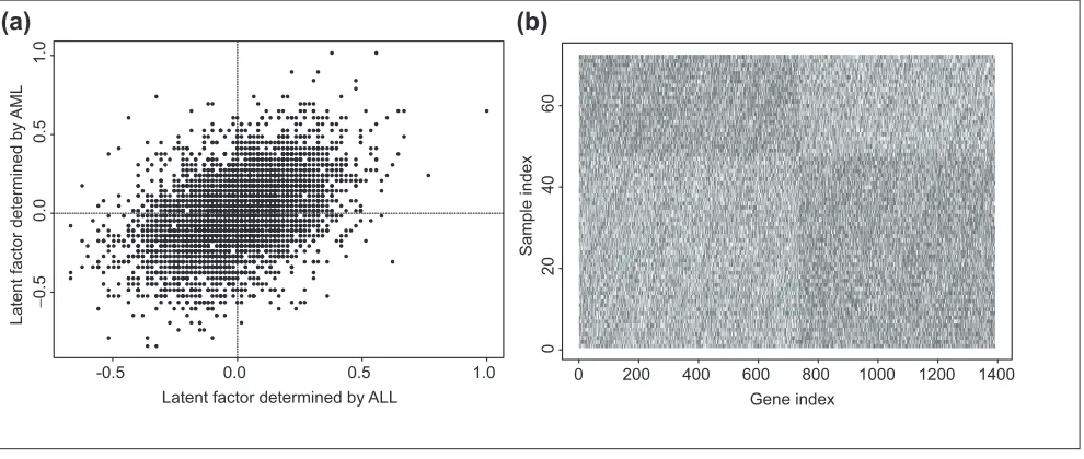
In order to see the difference of gene expression between ALL and AML samples, the two estimated factors are plotted on the left in Figure 4. Genes in the upper left quadrant tend to have higher gene expression level in AML, but lower expres-sion level in ALL. On the other hand, genes in the lower right quadrant tend to higher gene expression level in ALL, but lower expression level in AML. The logarithm (base 10) of the gene expression levels of these genes are plotted on the right panel in Figure 4. Clearly, these genes are differentially expressed between the two type of the samples. Further examination indicates that all the 100 genes identified by the Wilcoxon rank-sum test are included in these genes.

Analysis of NCI60 dataset

Relating gene expression profiles to drug activities

[image:6.609.60.558.87.297.2]

Scherf et al. [4] reported the use of cDNA microarrays to assess gene expression profiles in a set of 60 human cancer cell lines that have been characterized pharmacologically by treatment with more than 70,000 different drug agents, one at time and independently. This dataset offers us a unique opportunity to relate variations in gene expression to the molecular pharmacology of cancer. The NCI60 set includes cell lines derived from cancers of colorectal (CO, seven cell lines), renal (RE, eight cell lines), breast (BR, eight cell lines), ovarian (OV, six cell lines), prostate (PR, two cell lines), lung (LC, nine cell lines) and central nervous system (CNS, six cell lines) origin, as well as leukemias (LE, six cell lines) and melanomas (ME, eight cell lines). In this analy-sis, we consider only the 90 drug subsets whose mecha-nisms of action is putatively understood, and their activity data are available from the Web. We used the 1,376 gene Figure 2

(a) Log (base 10) of gene expression levels of 100 genes chosen using the Wilcox rank sum tests for the leukemias dataset. Darker spots indicate higher expression levels. The first 47 samples along the x-axis are ALL, the next 25 samples are AML. Genes are selected to best separate the two types of leukemias. (b) Plot of two latent factors estimated using the Rasch model for all 72 samples based on their gene expression profiles over 100 genes selected.

Sample index

Gene

index

0 20 40 60

0

204

06

08

0

10

0

−2 0 2 4

−

2

−

1

0

123

Latent factor 1

Latent

factor

2

ALL AML

(7)

subset along with 40 individually assessed targets for the present analysis. These subset was selected by selective filters used in [4]. These 90 drugs are listed in Table 1 of [4]. They applied the clustering methods to cluster cell lines basing on both gene expression profiles, and the drug

expression profiles. The phenotype of interest is chemother-apeutic susceptibility, as measured by -log GI50, where GI50 measures the dose needed to cause 50% growth inhibition. We first cluster the 1,476 genes using the model-based clus-tering method described previously using the original data

comment

reviews

reports

interactions

information

[image:7.609.55.556.87.291.2]

Figure 3

(a) Estimated latent factor and its 99% confidence interval for each gene based on its expression profile over the ALL samples. (b) Estimated latent factor and its 99% confidence interval for each gene based on its expression profile over the AML samples. For each plot, genes are ordered in the increasing order of the estimated latent factor. Genes between the two vertical lines are those whose expression levels are not significantly different. For a given leukemia type, genes with 99% confidence interval of the estimated latent factor not including zero show significantly different expression from those genes with 99% confidence interval of the estimated latent factor including zero.

Gene index

0 1000 2000 3000 4000

−

1.0

−

0.5

0.0

0.5

1.0

1.5

Gene index

Value

of

latent

factor

Value

of

latent

factor

0 1000 2000 3000 4000

−

1.5

−

1.0

−

0.5

0.0

0.5

1.0

1.5

(a)

(b)

Figure 4

(a) Estimated latent factors for each gene using ALL and AML samples. Genes in the upper left quadrant tend to be

overexpressed in the AML samples, but underexpressed in the ALL samples, and genes in the lower right quadrant tend to be overexpressed in the ALL samples, but underexpressed in the ALL samples. (b) Log (base 10) of gene expression levels for genes differentially expressed between ALL and AML samples.

Gene index

Sample

index

0 200 400 600 800 1000 1200 1400

02

0

40

60

(a)

(b)

Latent factor determined by ALL

Latent

factor

determined

by

AML

-0.5 0.0 0.5 1.0

−

0.5

0.0

0.5

[image:7.609.60.555.472.682.2]

(8)

of the log-ratios. The BIC scores in the upper left panel of Figure 5 indicate that there are four gene clusters, with 307, 312, 323 and 474 genes in each cluster, respectively. As a comparison, we also applied the hierarchical clustering method to cluster these genes. The dendrogram shown in the upper right plot of Figure 5 also indicates four gene clusters. For each cell line, a latent factor is estimated using the RM, based on the gene expression levels of the genes in each of the four clusters. To fit the RM, we discretize the gene expression levels into four categories using the quar-tiles. The same analysis was also done with eight catagories, and the results are the same. The lower left plot of Figure 5 shows the levels of these four latent factors sorted by cancer types. In general, cell lines with the same origin tend to have similar levels of the latent factors; therefore, these factors can be used for discriminating among the nine dif-ferent cell lines. However, for the third latent factor, the cell lines MDA-MB-435 (derived from the pleural effusion of a patient with breast cancer) and its Erb/B2 transfectant MDA-N have similar levels to those of latent factors esti-mated for the melanoma cell lines. To verify the utilities of these latent factors in clustering cell lines, we performed the hierarchical clustering analysis based on these four factors (see lower right plot in Figure 5). We note that the two breast cancer cell lines are clustered together with melanomas. Hierarchical clustering analysis using all the genes also resulted in clustering these two cell lines with melanomas. In general, cell lines of the same origin are clustered together on the basis of the four latent factors estimated with the RM. The clustering result of the cell lines using these four factors are similar to the clusters obtained using all the genes (see [4]).

Each of the 60 cell lines is now characterized by four differ-ent latdiffer-ent factors, where each latdiffer-ent factor is estimated based on the expression profiles of the genes in each of the four clusters. It would be interesting to relate these four latent factors to the drug activity patterns as measured by -log GI50across the 60 cell lines. For a given drug, we first performed a simple linear regression analysis treating the drug activity as response variable and using one of the four latent factors as a predictor, and obtained the parameter estimate of gin the following model:

drug activity = m+ gx latent factor.

The left panel of Figure 6 shows the estimated g value together with point-wise 99% confidence interval for each of the 90 drugs using one of the latent factors as a predictor. The variance of the regression parameter band the 99% con-fidence interval was estimated using the bootstrap proce-dure, where 50 resamples of genes in each cluster and 50 resamples of samples were used. For each latent factor, greater positive parameter estimate implies that higher gene expression level in a given gene cluster corresponds to a higher drug activity. For a given latent factor, drugs with 99% confidence interval of the estimated g parameter not including zero are those whose activities are related to genes which determine this latent factor.

In order to relate the drug activity of a given drug to all the four latent factors, we performed multiple linear regres-sion analysis where drug activity for a given cell line was treated as a response variable, and the four latent factors were treated as the predictors. The right plot of Figure 6 shows the estimates of the parameters in the multiple regression model for each of the 90 drugs. This plot can be used for selecting drugs that are related to gene expression profiles. For example, only drugs with at least one large parameter estimate are important for further study, as only for these drugs, their activity levels are related to gene expression profiles.

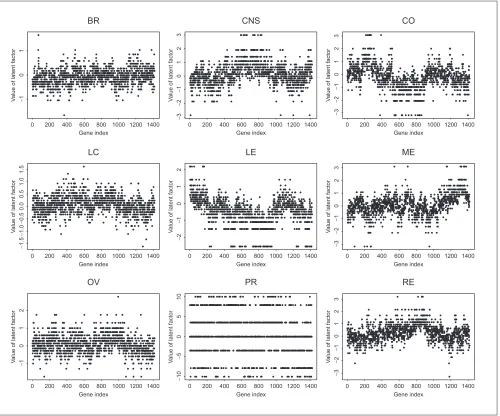
Identifying genes differentially expressed in different cell lines It is also interesting to identify genes that are over- or under-expressed relative to other genes for a given cell line type. Using the RM, we treat genes as persons and cell line samples as different items, and estimate the latent factor for each gene based on its expression profiles over all the samples of a given cell line type. Figure 7 shows the esti-mated latent factor for each gene based on the gene expres-sion profiles over each of nine different cell lines. These estimated latent factors provide a summary of gene expres-sions over different cell lines. Clearly, the gene expression profiles are different across different cell line types.

For a given cell line type, we can also infer which genes are over- or underexpressed compared to other genes based on the estimated latent factors. Figure 8 shows the estimated Table 1

Genes over- and under-expressed in breast-cancer cell line

Overexpressed

TP53 tumor protein p53 (Li-Fraumeni syndrome) Antiquitin

Elongation factor TU, mitochondrial precursor Human mRNA for collagen-binding protein 2

Homo sapiensintermediate conductance calcium-activated potassium channel

H. sapiensmRNA for phosphoenolpyruvate carboxykinase H. sapiensinactive palmitoyl-protein thioesterase-2i (PPT2) mRNA H. sapienslysosomal neuraminidase precursor

Underexpressed

Tumor-associated antigen CO-029

Probable trans-1,2-dihydrobenzene-1,2-diol dehydrogenase Human fetus brain mRNA for membrane glycoprotein M6

Human mitochondrial 1,25-dihydroxyvitamin D3 24-hydroxylase mRNA H. sapiensDAP-kinase mRNA

(9)

latent factor and the point-wise 99% confidence interval for each gene for each of the nine cell line types. For a given cell line, genes with 99% confidence interval of the estimated latent factor not including zero show significantly different expression from those genes with 99% confidence interval of the estimated latent factor including zero. For example, for breast cancer cell line, the method identified 15 genes or expressed sequence tags (ESTs) that are relatively overex-pressed (the estimated latent factor is greater than zero, and is significant at the 0.01 level) and 23 genes or ESTs that are relatively underexpressed (estimated latent factor is less than zero, and is significant at the 0.01 level) in the breast cancer cell lines. Table 1 lists the known genes. Interestingly, we note that genes that are overexpressed include p53, and genes that are underexpressed include that for tumor-associ-ated antigen CO-029. On the basis of our analysis, all other genes have similar gene expression level in the breast cancer

cell line. Genes that are over- or underexpressed in other types of cell line can be similarly identified.

Discussion

We have described two different formulations of the RM for relating gene expression data to phenotypes. The RM provides a probabilistic model to describe the observed gene expression patterns. The first formulation can be used for cancer class prediction, and for identifying clusters of genes with similar expression profiles that are related to drug responses. The method is based on a combination of cluster-ing analysis, the RM and the regression analysis. The second formulation can be used for identifying differentially expressed genes from different types of sample. We applied this method to a publicly available leukemia dataset to demonstrate the application of the proposed method for

comment

reviews

reports

interactions

information

[image:9.609.54.555.88.471.2]

Figure 5

(a) BIC scores as a function of the number of clusters for the NCI60 dataset. (b)Dendrogram showing hierarchical

clustering of the genes. (c)Four latent factors estimated by using the Rasch model. The cancer indexes are sorted by cancer types as CNS, BR, RE, LC, ME, PR, OV, CO, LE (see text for abbreviations). (d)Dendrogram showing hierarchical clustering of cell lines based on four latent factors estimated by using the Rasch model.

Number of clusters

BIC

2 4 6 8 10 12 14

−

2.34

x

10

5

−

2.30

x

10

5

−

2.26

x

10

5

CNS

BR

CNS

BR RE

RE RE

RE

RE RE

RE

LC

ME

PR

RE

PR

LC

LC OV BR

OV

LC

BR ME

ME

ME BR BR ME

ME ME

ME

OV

BR

LC

CO

CO CO

CO

LC

LE

LE LE

0.0

0.5

1.0

1.5

2.0

2.5

02

468

10

Latent factor 1

Cancer index

Estimated

latent

factors

0 10 20 30 40 50 60

−

0.6

-0.2

0.2

Latent factor 2

Cancer index

Estimated

latent

factors

0 10 20 30 40 50 60

−

0.5

0.0

0.5

1.0

Latent factor 3

Cancer index

Estimated

latent

factors

0 10 20 30 40 50 60

−

0.5

0.0

0.5

1.0

Latent factor 4

Cancer index

Estimated

latent

factors

0 10 20 30 40 50 60

−

2.0

−

1.0

0.0

1.0

(a)

(b)

(10)

[image:10.609.57.554.86.672.2]

Figure 6

(a) Parameter estimate and the bootstrap 99% confidence interval of simple linear regression parameter gfor each of the 90 drugs and for each latent factor. For a given latent factor, drugs with 99% confidence interval of the estimated gparameter not including zero are those whose activities are related to genes which determine this latent factor. (b)Parameter estimates (for each drug, four regression coefficients for four latent factors) of multiple linear regression for each of the 90 drugs.

Latent factor 1

Drug index(sorted)

Gamma

0 20 40 60 80

−

2

024

Latent factor 2

Drug index(sorted)

Gamma

0 20 40 60 80

− 2 − 10 1 2

Latent factor 3

Drug index(sorted)

Gamma

0 20 40 60 80

− 1.5 − 0.5 0.5 1.5

Latent factor 4

Drug index(sorted)

Gamma

0 20 40 60 80

− 1.0 0.0 0.5 1.0 1 1 1 1 11 1 1 1 1 1 1 1 1 1 1 11 1 1 1 1 1 1 1 1 111 11 1 1 1111 11₁₁

1 11 111 11 1 1 1 11 1 111 1 111 1 1 1 1 1 1 1 1

11111₁₁

1 11 11 1 11 111 1 1 2 2 222 22 2 2 2 2 2 22 2 2 2 22 22 2 2 222 2 2 2 2 2 2 2 2 2 22 2 22 222222 2 2 22 2 222 2 2 2 2 2222 2 2 2 222 2 22

222 22

22₂2 22 22 2 2 22 2 2 333 3 33 3 3 3 3 3 33 3 3 3 3 33 3 333 3 33 3 3 333 3 3 3 3 3 3 3 33 333 33 3 3 3 33 3 3 3 3 3 33₃₃₃₃₃₃

33

333333333₃₃ 3 3 3 333₃ 3 33 33 3 3

444 444444 4 4 4 4 44 4 4 4 4 4 4 44 4 4 4 44 44 4 44 4 444 4444 44

44₄444 4 4 4 4 4 4 4 4 44 444 4 4 4 44 4 44 444444 4 4 4 4 4 44

44444

4 4

Drug index

Coef

ficients

0 20 40 60 80

(11)

class prediction. We also applied this method to an analysis of the NCI60 data to show that the method can also be applied to other phenotypes.

The method introduced here has several advantages. First, it provides a probabilistic model for describing the gene expression patterns. These models are used to reduce the complexity of the raw data and offer a certain degree of sim-plification. In contrast to most of the currently available methods for gene expression data, such as principal compo-nent analysis, the model used here provides a non-linear method for dimension reduction. Second, compared with traditional density-based models, the method is more robust to outliers, as it uses ranks rather than actual expression levels. There is a long sequence of steps in the laboratory as

well as in the image analysis before a single number is pro-duced for an expression level, and there are many potential sources of error. Methods that use ranks rather than the original measured gene expression data are also advocated by A Tsodikov, A Szabo and D Jones (unpublished data) and Park et al. [21]. Third, in contrast to clustering methods for simultaneously clustering both genes and samples, the model-based approach allows formal estimates of the vari-ance and therefore facilitates formal tests of null hypotheses and assignments of confidence intervals.

There are several limitations to the proposed approach. First, in order to apply the RM, the gene expression levels are dis-cretized. It is clear that by discretizing the measured expres-sion levels we are losing information. Certainly, additional

comment

reviews

reports

interactions

information

[image:11.609.56.556.87.503.2]

Figure 7

Estimated latent factor for each gene and each cell line type. Genes are in the same order across different cell lines to show that genes have different values of the latent factors, and therefore, different expression profiles across different cell line types. See text for abbreviations.

BR

Gene index

Value

of

latent

factor

0 200 400 600 800 1000 1200 1400

−

10

1

CNS

Gene index

Value

of

latent

factor

0 200 400 600 800 1000 1200 1400

−

3

−

2

−

1

0

123

CO

Gene index

Value

of

latent

factor

0 200 400 600 800 1000 1200 1400

−

3

−

2

−

1

012

3

LC

Gene index

Value

of

latent

factor

0 200 400 600 800 1000 1200 1400

−

1.5

−

1.0

−

0.5

0.0

0.5

1.0

1.5

LE

Gene index

Value

of

latent

factor

0 200 400 600 800 1000 1200 1400

−

2

−

10

1

2

ME

Gene index

Value

of

latent

factor

0 200 400 600 800 1000 1200 1400

−

3

−

2

−

1

0123

OV

Gene index

Value

of

latent

factor

0 200 400 600 800 1000 1200 1400

−

10

1

2

PR

Gene index

Value

of

latent

factor

0 200 400 600 800 1000 1200 1400

−

10

−

50

5

10

RE

Gene index

Value

of

latent

factor

0 200 400 600 800 1000 1200 1400

−

3

−

2

−

1

0

(12)

information is present in the level of gene expression, but normalization or scaling errors across subjects or slides make it difficult to determine the precision of these numbers. We believe that discretization provides a reason-ably unbiased approach for dealing with this type of data. For both the leukemia and NCI60 datasets, we fitted the RMs by discretizing the gene expression levels into both four and eight categories, and obtained essentially the same con-clusions. Of course, the more categories we use, the closer are the discretized data to the real continuous data. However, this will introduce more parameters to the model. Second, this approach assumes that genes can be clustered into several subgroups based on their expression profiles over samples. This might not be true for some studies. In this case, we can consider all the possible clusters of genes in

a step-wise regression analysis as proposed by Hastie et al. [22]. Third, we used the bootstrap resampling procedure to estimate the variance of the regression parameter bafter we have clustered genes into several classes. This procedure does not account for possible variability associated with the clustering step, and therefore, the bootstrap variance esti-mates are likely to be underestimated.

[image:12.609.57.558.86.491.2]

In our proposed method, the clustering, the Rasch modeling and the regression analysis are done separately. Important research for the future is to take a joint likelihood approach that can combine all three steps to obtain better estimates of the number of clusters, the latent factors and the regres-sion parameters. This kind of mixture RM provides a natural framework for unifying statistical inference and Figure 8

Estimated latent factor and the associated point-wise 99% confidence interval for each gene and each cell line type. For cell line type, the genes are sorted by the estimated value of the latent factor. For a given cell line, genes with 99% confidence interval of the estimated latent factor not including zero show significantly different expression from those with 99% confidence interval of the estimated latent factor including zero. See text for abbreviations.

BR

Gene index

Value

of

latent

factor

0 200 400 600 800 1000 1200 1400

−

3

−

2

−

10

1

2

3

CNS

Gene index

Value

of

latent

factor

0 200 400 600 800 1000 1200 1400

−

4

−

20

2

4

6

CO

Gene index

Value

of

latent

factor

0 200 400 600 800 1000 1200 1400

−

6

−

4

−

20

2

4

6

LC

Gene index

Value

of

latent

factor

0 200 400 600 800 1000 1200 1400

−

3

−

2

−

10

1

2

LE

Gene index

Value

of

latent

factor

0 200 400 600 800 1000 1200 1400

−

4

−

2

024

ME

Gene index

Value

of

latent

factor

0 200 400 600 800 1000 1200 1400

−

6

−

4

−

20

2

4

6

OV

Gene index

Value

of

latent

factor

0 200 400 600 800 1000 1200 1400

−

20

2

4

PR

Gene index

Value

of

latent

factor

0 200 400 600 800 1000 1200 1400

−

15

−

10

−

50

5

10

15

RE

Gene index

Value

of

latent

factor

0 200 400 600 800 1000 1200 1400

−

6

−

4

−

20

2

4

(13)

clustering. We are currently carrying out research in this direction. In conclusion, we demonstrate here the potential application of the RMs in analysis of gene expression data. RMs provide a probability model for describing gene expression profiles measured over different samples or over different times. We are currently exploring various other formulations of the microarray gene expression problems in the framework of the RMs, including class discovery in cases of hidden taxonomies based on the estimated latent factors using the RM.

Acknowledgements

This research is supported in part by an NIH grant (ES09911) and a UC Davis Health System Research Award grant.

References

1. Golub TR, Slonim DK, Tamayo P, Huard C, M Caasenbeek M, Mesirov JP, Colle Hr, Loh ML, Downing JR, Caligiuri MA, et al.: Mol-ecular classification of cancer: class discovery and class pre-diction by gene expression monitoring. Science 1999, 286:531-537.

2. Alon U, Barkai N, Notterman DA, Gish K, Ybarra S, Mack D, Levine AJ: Broad patterns of gene expression revealed by clustering analysis of tumor and normal colon tissues probed by oligonucleotide arrays. Proc Natl Acad Sci USA 1999, 96: 6745-6750.

3. Alizadeh A, Eisen M, Davis RE, Ma C, Lossos I, Rosenwal A, Boldrick J, Sabet H, Tran T, Yu X, et al.: Distinct types of diffuse large B-cell lymphoma identified by gene expression profiling. Nature 2000, 403:503-511.

4. Scherf U, Ross DT, Waltham M, Smith LH, Lee JK, Kohn KW, Rein-hold WC, Myers TG, Andrews DT, Scudiero DA, et al.: A cDNA microarray gene expression database for the molecular pharmacology of cancer.Nat Genet2000, 24:236-244.

5. West M, Nevins J, Marks JR, Spang A, Zuan H: Bayesian Regression Analysis in the “Large p, Small n” Paradigm with Application in DNA Microarray Studies. Technical Report. Duke University, 2000. This report is available at [http://www.isds.duke.edu]

6. Rasch G: Probabilistic Models for Some Intelligence and Attachment Tests. Copenhagen: Danish Institute of Educational Research, 1960. 7. Fischer GH, Molenaar IW (eds): Rasch Models: Foundations, Recent

Developments, and Applications. New York: Springer; 1995.

8. Jaen J, Alvarez P, Roman P, Alonso E, Bayo E, Salas C: Rasch model: An available method for measuring the quality of life of cancer patients.Oncologia (Madrid)1994. 17:49-58.

9. Sheehan TJ, DeChello LM, Garcia R, Fifield J, Rothfield N, Reisine S: Measuring disability: application of the Rasch model to activities of daily living (ADL/IADL). J Outcome Measurement 2000-2001, 4:681-705.

10. Fraley C, Raftery AE: How many clusters? Which clustering method? Answers via model-based cluster analysis.Computer J1998, 41:578-588.

11. Wen X, Fuhrman S, Michaels GS, Carr DB, Smith S, Baker JL, Somogyi R: Large-scale temporal gene expression mapping of central nervous development. Proc Natl Acad Sci USA 2000, 95:334-339.

12. Eisen M, Spellman PT, Brown PO, Botstein D: Cluster analysis and display of genome-wide expression patterns.Proc Natl Acad Sci USA1998, 95:14863-14868.

13. Spellman PT, Sherlock G, Zhang MQ, Iyer VR, Anders K, Eisen MB, Brown PO, Botstein D, Futcher B: Comprehensive identification of cell cycle-regulated genes of the yeast Sacccharomyces cerevisae by microarray hybridization. Mol Biol Cell 1998, 9:3273-3297.

14. Tavazoie S, Hughes JD, Campbell, MJ, Cho RJ, Church GM: System-atic determination of genetic network architecture. Nat Genet1999, 22:281-285.

15. Masters GN: A Rasch model for partial credit scoring. Psy-chometrika1982, 47:149-174.

16. Andersen EB: Polytomous Rasch models and their estimation. In Rasch Models: Foundations, Recent Developments, and Applications. Edited by Fischer GH, Molenaar IW. New York: Springer; 1995. 17. McLachlan G, Basford K: Mixture Models: Inference and Applications to

Clustering. New York: Marcel Dekker; 1988.

18. Hartingan JA, Wong MA: Algorithm AS136: A k-means cluster-ing algorithm.Appl Statistics1979, 28:10-108.

19. Schwarz G: Estimating the dimension of a model. Annls Statistics 1978, 6:461-464.

20. Efron B: The Jacknife, the Bootstrap, and Other Resampling Plans. Philadelphia: Society for Industrial and Applied Mathematics, 1982. 21. Park PJ, Pagano M, Bonetti M: A nonparametric scoring

algo-rithm for identifying informative genes from microarray data.Proc Pacific Symp Biocomput2001, 6:52-63.

22. Hastie T, Tibshirani R, Botstein D, Brown P: Supervised harvest-ing of expression trees. Genome Biol 2001, 2: research003.1-003.12.