ANALOG CIRCUIT FAULT DIAGNOSIS METHOD BASED
ON PARTICLE SWARM NEURAL NETWORK
1
Baoru Han, 2Hengyu Wu(Corresponding Author),3Shixiang Liu
1-3
Department of Electrical Engineering, Hainan Software Profession Institute,Qionghai, China
E-mail: [email protected],
ABSTRACT
With the combination of particle swarm optimization and neural network, this paper presents a kind of analog circuit fault diagnosis method based on particle swarm neural network. In the training process, the linear decreasing inertia weight particle swarm algorithm optimized BP network’s initial weights and initial threshold, adaptive learning rate and additional momentum BP algorithm adjusted the weights and threshold of BP neural network, which makes the best of particle swarm algorithm and BP algorithm local search advantage to overcome the traditional BP algorithm converging slowly and falling into the limitations of local weights easily. Simulation results show that this diagnostic method can be used for tolerance analog circuit fault diagnosis, with a high convergence rate and diagnostic accuracy.
.
Keywords: Fault diagnosis, Particle swarm neural network, Linear decreasing inertia weight, Analog circuits
1. INTRODUCTION
Modern society, electronic devices or systems are widely used in various scientific and technological fields, the industrial production sector as well as in people’s daily life, and the reliability of electronic equipment has a direct impact on the efficiency of production, systems, equipment and human lives and safety. With the increasingly widespread use of electronic equipment, whether in the production phase of the equipment or the application stage, the circuit fault diagnosis is put forward for the urgent request, urging people to study the new effective diagnostic techniques to further improve the reliability of electronic equipment [1]. At present, the overwhelming majority of faults in electronic equipment come from analog circuits. Therefore, in a sense, the reliability of analog circuit determines the reliability of electronic equipment system. With the rapid development of electronic technology, analog circuit fault diagnosis technology is badly needed whether in the stage production of electronic equipment or the application process. Since the seventies of the last century, analog circuit fault diagnosis has been the one of the hot concerns in the international academic community, called the frontier of modern circuit theory [2].
Neural network storage information in a distributed manner has strong fault tolerant ability,
self-organizing and self-learning ability, the ability to deal with fuzzy information, making it a kind of effective analog circuit fault diagnosis method
[3-6]. Particle Swarm Optimization [7] simulates birds
flying foraging behavior to achieve the optimal
objective through collective collaboration between
bird groups. In the PSO system, each candidate
solution is referred to as a “ particle” ( Particle ), a plurality of particles coexist, collaborative optimization ( approximate birds for food ), each particle according to its own “experience” and the adjacent particle swarm optimal “experience ” in the problem space to better position “ flight “, to
search the optimal solution. Compared with other
optimization algorithm, particle swarm optimization algorithm is simpler and easier without many parameters adjustment [8-9].
optimization and BP algorithm combining hybrid algorithm. In the training process, the linear decreasing inertia weight particle swarm algorithm optimized BP network’s initial weights and initial threshold, adaptive learning rate and adjusted the network weights and threshold in additional momentum BP algorithm. The hybrid algorithm is applied to tolerance analog circuit fault diagnosis, with a short training time, calculating advantages of high accuracy, global convergence, effectively reduction of the miscarriage of justice, and the missing of the situation to improve the accuracy and rapidity of fault diagnosis.
2. PARTICLE SWARM OPTIMIZATION ALGORITHM
Particle swarm optimization algorithm, inspired by social behavior of bird flocking, is a population based stochastic optimization technique developed by Dr. Eberhart and Dr. Kennedy in 1995[7]. PSO shares many similarities with evolutionary computation techniques such as Genetic Algorithms (GA). The system is initialized with a population of random solutions and searches for optima by updating generations. In PSO, the potential solutions, called particles, fly through the problem space by following the current optimum particles. Each particle keeps track of its coordinates in the problem space which are associated with the best solution (fitness) it has achieved so far. (The fitness value is also stored.) This value is called gbest. Another “best” value tracked by the particle swarm optimizer is the best value, obtained by any particle in the neighbors of the particle. This location is called 1best. When a particle takes all the population as its topological neighbors, the best value is a global best and is called gbest.
In particle swarm optimization algorithm, each particle can be considered as a point in the solution space. If the group size of particles is N, then the i-th (i = 1, 2, ..., N) i-the location of i-the particles can
be expressed as xi. It has experienced the “best”
position is denoted as pbest [i]. Its speed is
expressed by vi. The gbest [i] represents
populations of the “best” particle location. Particle
i will update their speed and position according to the following formula (1) and formula (2).
(
)
(
g
x
)
c
x
p
c
v
v
i best
i best i
i
i rand
i rand
w
− ∗
∗ +
− ∗
∗ + ∗ =
] [ ()
] [ ()
2
1 (1)
v
x
x
i= i+ i(2)
Where c1, c2 are constants called learning factors,
usually c1 = c2 = 2; rand () is a random number in
[0, 1], w is the inertia weight (inertia weight). The
formula consists of three parts. The first part is the particle's previous speed, indicating the current state of the particles, play a balanced role of a global search and a local search; the second part is cognitive portion, expressed reflection of the particles themselves, so that the particles have a strong enough global search capability, to avoid local minima; third part is the social part (social Modal) reflects the information-sharing between
the particles. The three parts determines the search
ability of particle space. In addition, the particles
constantly adjust their position according to the speed, but also limited by the maximum velocity
(Vmax). When vi exceeds Vmax, vi will be limited
to Vmax.
3. LINEARLY DECREASING INERTIA WEIGHT
Particle swarm optimization algorithm structure is simple, running fast. In the optimization process, if a particle is to find a local advantages, other particles will quickly to the mobile, duo to which it will fall into the local optimal solution, with no finding global optimal solution of the opportunity. In order to reduce their falling into local opportunities, we must always keep the particles have a certain diversity, thereby introducing improved particle swarm optimization (abbreviated: IPSO) algorithm [12-13]. This paper uses improved
inertia weight algorithm. The choice of fixed
weights is to select a constant inertia weight unchanged during the optimization process. However, in practical applications, particle swarm optimization effect is not very ideal. This article began to study the impact of inertia weight w to optimize performance, found that the larger the value of w is conducive to jump out of local minima, and smaller w values conducive to the
convergence of the algorithm. So this paper adopts
a linear decreasing inertia weight algorithm. Inertia
weight linearly decreasing is decided by the number
of iterations of the algorithm. In the early stage,
the algorithm uses a larger inertia weight, with strong global search ability. In the late stage, the algorithm uses a smaller inertia weight in order to
improve the local search ability. It is a kind of
inertia weight selection method, which can achieve an optimal balance between global search and local
search. Inertia weight value is calculated as
iter iter
w
w
w
w
max min max max − × −
=
(3)
Among them, wmax and wmin are the initial and
final values of the inertia weight, and 0.1 wmin <
wmax≤ 0.9. Maxiter and iter are the maximum
number of iterations and the current algebra of the algorithm.
4. BP NEURAL NETWORK
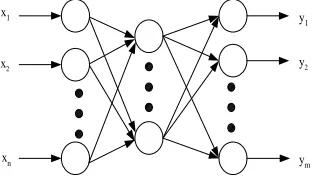
[image:3.612.331.526.309.417.2]BP network structure is similar to the multilayer perception. It is a multi-layer feed forward neural network. BP neural network model is shown in figure 1. The neural network has a strong nonlinear mapping ability, fault tolerance and generalization ability. The kolmogorov theorem can be learned with a single hidden layer perception can map all continuous functions. Therefore in this paper a single hidden layer BP neural network was chosen for analog circuit fault diagnosis.
x1 x2 xn y1 y2 ym
Figure 1: BP neural network model
The output of the network in the first layer is the second layer of the network input. The output of the second layer of the network is the input of the third layer of the network. The number of neurons in each layer may be different. There is no coupling between the neurons in the same layer on the connection relationship. Information from the input layer to start one-way propagation between the layers, through hidden layer neurons, finally reaches the output layer neurons. Be in the back-propagation transfer function of the derivative calculation, so they requested that the transfer function of the BP neural network be differentiable. Therefore the sigmoid, tangent function and a linear function are often used to speed up the BP neural network training speed, to avoid falling into the local minimum, to improve the effectiveness of the algorithm, adaptive learning rate and the additional momentum BP algorithm. BP neural network is trained in batch mode. It is adaptive learning rate and the additional momentum BP algorithm that adjust the network weights.
BP neural network training specific steps are as follows.
(1) Determining the structure of BP neural network based on various learning parameters, including the momentum coefficient error parameters and adaptive learning rate parameters.
(2) Initialize the network weights, and set the initial value to the BP neural network.
(3) Calculate the hidden layer neurons in input and output.
(4) Calculate the output layer of the neural input and output.
(5) With the desired output and the actual output network, calculate the output layer neurons of the error.
(6) Adjust the weights of the network and the learning rate according to the adaptive learning rate and additional momentum BP algorithm, and set the next learning according to the adjusted rate of learning to learn. The formula is as follows:
( ) ) ( ) ( ) 1 ( ) 1
( mc wn
n w n E n mc n
w + ∆
∂ ∂ −
= +
∆ η( ) (4)
) ( ) ( ) ( ) 1 ( ) 1
( mc bn
n b n E n mc n
b + ∆
∂ ∂ −
= +
∆ η( ) (5)
> + < + = + ) ( ) 1 ( ), ( ) ( ) 1 ( ), ( ) 1 ( n E n E n n E n E n n βη αη
η (6)
η(n+1)=η(n) (7)
mc
is momentum coefficient.η
(n) is theadaptive learning rate.
α
,β
are learning rate andadjustment coefficient respectively.
(7) Select the next input sample data to the BP neural network, return to step (3), until all of the sample data is ended. And cumulate errors, and finally get all the learning sample errors with a complete training.
(8) View the training errors and the times of iterations. If the errors reach the required maximum or the set times of iterations, end the learning process. Otherwise, return to step (2) until the global error function in network learning is less than a predetermined set of a minimal value.
(9) The end of learning.
4. PARTICLE SWARM NEURAL NETWORK
[image:3.612.125.281.337.434.2]determined according to the input sample and desired output, and thus determines the spatial dimension of particle swarm PSO algorithm. Particle Swarm spatial dimension is the sum of the number of BP neural network weights and threshold. Mean square error function between the desired output and the actual output of BP neural network is taken as the fitness function of PSO algorithm. Optimal initial weights and initial threshold value of neural network are obtained by PSO algorithm optimization search. Measure the fitness of each particle is the mean square error between the expected and actual output value of BP neural network.
Fitness function formula is as follows.
(
)
21 1
1
∑∑
−
= =
= P
p Q
q
y
d
pq pqPQ
mse (8)
Among them, mse is the fitness value of each
particle; P is the total number of the training sample
set; Q is the number of output neurons; the dpq is
p-th samples of p-the q-p-th output neuron ideal output
value; the ypq is p-th sample of the q-th actual
output value.
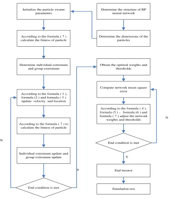
Particle swarm neural network training algorithm flow chart is shown in figure 2.
Determine the structure of BP neural network
Determine the dimensions of the particles
Initialize the particle swarm parameters
According to the formula ( 7 ) calculate the fitness of particle
Determine individual extremum and group extremum
According to the formula ( 1 ), formula (2 ) and formula ( 3 ) update velocity and location
According to the formula ( 7 ) to calculate the fitness of particle
Individual extremum update and group extremum update
End condition is met
Compute network mean square error
According to the formula ( 4 ), formula (5 ) ,formula (6 ) and formula ( 7 ) adjust the network
weights and thresholds
End condition is met
End iterator
Simulation test Obtain the optimal weights and
thresholds
N
Y
N
[image:4.612.149.487.257.653.2]Y
Figure 2: Particle swarm neural network training algorithm flow chart
Hybrid particle swarm neural network training algorithm is divided into two stages. Early in training, the use of a linear decreasing inertia weight particle swarm algorithm global search
ability of local search, using adaptive learning rate and additional momentum BP algorithm to continue to train the neural network.
5. SIMULATION
5.1 Fault Model
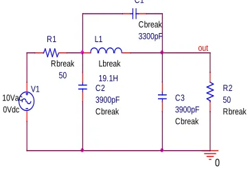
This article select RLC band pass filter circuit as an example for fault diagnosis simulation. The RLC band-pass filter circuit is shown in figure 3.It is composed of 2 resistors, 3 capacitors and 1 inductance components RLC. Resistance tolerance is 8%. Inductance and capacitance tolerance is 9%, 10%respectively.
Cbreak
C1 3300pF
Cbreak
C2 3900pF
Cbreak
C3 3900pF R1
Rbreak
50
R2
Rbreak
50 V1
10Vac 0Vdc
0
out
Lbreak
L1
[image:5.612.107.289.265.392.2]19.1H
Figure 3 :RLC band-pass filter circuit
Faults are divided into two categories: hard fault (component of short circuit or open circuit); soft fault (element parameter exceeds a predetermined tolerance range). In this paper, it is only considered the hard failure. The hard fault models use a resistor bridge. Due to the adoption of the output frequency in response to fault diagnosis in analog circuits so not every fault element can effectively diagnosis. Because some elements of parameter changes on the output frequency response is very small. So in the diagnosis of anterior put sensitivity analysis to the RLC band-pass filter circuit. Because of C1, C2, L1 and R1 change circuit frequency response output influence therefore, selecting C1 open, C2 open circuit, short circuit or C1 for short circuit to L1, R1 short-circuit the 4 fault. The desired output respectively normal state (000), C1 open circuit (001), C2 open circuit (010), C1 or L1 short circuit short circuit (011) and R1 (100) short circuit.
5.2 Neural Network Training and Testing
For every kind of fault, running the 60 Monte-Carlo analyses, the output waveform in the data stored in the.Txt text, and then using MATLAB software to automatically obtain accurate fault sample data, principal component analysis,
structure sample set.
Particle swarm neural network was used for RLC band-pass filter circuit fault diagnosis. Particle swarm neural network parameters are set as
follows. Learning factor c1 = c2 = 2. The initial
value of the inertia weight wmax = 0.90, the final
value of the inertia weight Wmin = 0.30. Particle
fitness value mse = 0.17. Particle swarm the
number of iterations is 50. The population of the number of particles is 5. Input neuron number is 6. The number of hidden neurons in 40.The output neuron number is 3.Hidden layer neuron transfer function using tansig. Output layer neurons of the transfer function using logsig. Expected error is 0.0265, the number of training is the 5000 epochs.
After setting the above parameters, the particle swarm neural network is trained with a training set of sample. The best individual fitness value change process is shown in figure 4. Figure 5 is the particle swarm neural network training error curve. Particle swarm neural network after training, in order to test the performance of the network, using the test set for testing. The test samples in the diagnosis results of the average error are 0.0216. Particle swarm neural network can accurately identify the circuits of 5 types of fault.
0 5 10 15 20 25 30 35 40 45 50
0.16 0.18 0.2 0.22 0.24 0.26 0.28 0.3 0.32 0.34 0.36
iterations
B
es
t i
ndi
v
idual
f
it
nes
s
v
al
ue
Figure 4: Particle swarm algorithm optimization process
0 10 20 30 40 50 60 70
10-4 10-3 10-2 10-1 100
Epochs
M
ean S
quar
ed E
rr
or
(
m
s
e)
Training for 70 Epochs
0 20 40 60 80 100 120 140 10-4
10-3 10-2 10-1 100
Best Training Performance is NaN at epoch 140
M
ean S
quar
ed E
rr
or
(
m
s
e)
Epochs
Train Best Goal
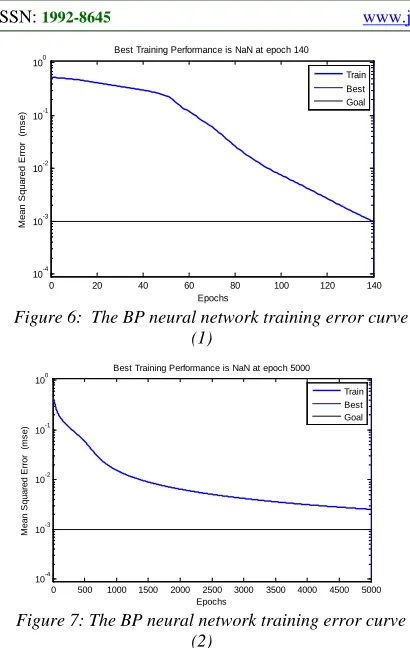
Figure 6: The BP neural network training error curve (1)
0 500 1000 1500 2000 2500 3000 3500 4000 4500 5000 10-4
10-3 10-2 10-1 100
Best Training Performance is NaN at epoch 5000
M
ean S
quar
ed E
rr
or
(
m
s
e)
Epochs
Train Best Goal
Figure 7: The BP neural network training error curve (2)
For comparison purposes, also using the gradient descent learning algorithm adaptive and learning rate and the additional momentum BP algorithm for BP neural network is trained, parameters related to the same, and training samples are identical. The training curves are as shown in figure 6 and figure 7. The test samples in the diagnosis results of the average error are 0.0496 and 0.0359. They can accurately identify the circuits of 5 types of fault.
To observe the simulation results, the particle swarm neural network training algorithm performance is relatively good, and has good convergence, in the 70 step it has converge to the desired error 0.001. Adaptive learning rate and the additional momentum BP algorithm error curve convergence is slower than the particle swarm neural network training error curve convergence rate, in about 140 steps to converge to the expected error 0.001. Ordinary gradient descent learning BP algorithm after the completion of the training times has not reached the expected error 0.001. Judging from the diagnostic accuracy, the particle swarm neural network average error is much smaller than the average error of the latter two.
6. CONCLUSIONS
This article describes a particle swarm neural
network analog circuit fault diagnosis method., The method takes the linear decreasing inertia weight particle swarm algorithm to optimize BP network's initial weights and initial thresholds, uses adaptive learning rate and additional momentum BP algorithm to adjusted the network weights and thresholds. In the case of the same learning samples, it has a short training time and calculated high precision. Simulation diagnostic results confirm this fault diagnosis method is correct and effective; there is a certain value in practical engineering. Particle swarm algorithm can also be optimized BP network structure and learning rules, it is worth further study.
ACKNOWLEDGMENT
The work is supported by the Natural Science Foundation of Hainan Province (No: 611127).
REFRENCES:
[1] Bandler J W, Salama A E, “Fault Diagnosis of
Analog Circuits”, Proceedings of the IEEE,
Vol. 73, No. 8, 1985, pp.1279-1327
[2] ARTUR R, ROMUALD Z, “Fault diagnosis of analog piecewise linear circuits based on
homogony”, IEEE Transactions on Instruments
and Measurement, Vol.51, No.4, 2002, pp. 876−881.
[3] Aminian F, “Analog Fault Diagnosis of actual
Circuits using Neural Networks”, IEEE
Transactions on Instrumentation and Measurement, Vol.51, No.3, 2002, pp. 544-550 [4] Stopjakova V, Malosek P, “Classification of
Defective Analog Integrated Circuits Using
Artificial Neural Networks”, Journal of
Electronic Testing Theory and Applications,
No.20, 2002, pp.25-37.
[5] Mohammadi K, “Fault Diagnosis of Analog Circuits with Tolerances by Using RBF and
BP Neural Networks”, Student Conference on
Research and Development Proceedings,
Vol.12, No.3, 2002, pp.317-321.
[6 ] Chen Guo, “Analysis of influence factors for forecasting precision of artificial neural
network model and its optimizing”, Pattern
Recognize & Artificial Intelligent , 2005 , Vol.18, No.5, 2005, pp.528- 534
[7] Kennedy J, Eberhart R, “Particle Swarm
Optimization”, IEEE on Networks, 1995,
[image:6.612.97.302.73.397.2][8] Eberhart R C, Kennedy J, “A New Optimizer
Using Particle Swarm Theory”, Proceeding of
Sixth International Symposium on Micro Machine and Human Science,Japan,1995
pp.39-43.
[9] Jiang Tao, ZHANG Yu-fang, Wang Yinhui,“An improved particle swarm algorithm in BP network applied research in
network”, Computer Science, Vol.33, No.9,
2006, pp.164-190.
[10] He W M,Wang P L, “Analog Circuit Fault Diagnosis Based on RBF Neural Network
Optimized by PSO Algorithm”, 2010
International Conference on Intelligent Computation Technology and Automation, 2010, pp.628-631.
[11] Gao Haibing, Gao Liang, Zhou Chi, “Particle swarm optimization based algorithm for
neural network learning”, Acta Electronica
Sinica, Vol.32, No.9, 2004, pp.1572-1574. [12] Song Naihua, Xing Qinghua, “A new
learning algorithm of BP network based on
particle swarm optimization”, Computer
Engineering, Vol.32, No.14, 2006, pp.181- 183.
[13] Shi Y, Eberhart R, “A modified particle
swarm optimizer”, IEEE World Congress on
Computation Intelligence , 1998 pp. 69- 73.