997
MAINTENANCE POLICY OPTIMIZATION FOR A
DETERIORATING SYSTEM WITH MULTI-FAILURES
1
HUANZHI FENG, 1LAIBIN ZHANG, 1WEI LIANG
1
College of Mechanical and Transportation Engineering, China University of Petroleum, Beijing 102249,
China
E-mail: [email protected]
ABSTRACT
For complex systems in modern industry system, optimal maintenance policy is difficult to determine concerned balance between risks and costs because numerical elements have effectives to each others. To solve this critical problem, this paper presents an optimal maintenance model for a multi-state deteriorating system subject to multi-failures. The system process is modeled as a semi-Markov process. The model has considered both multi-condition states and multi-failure states of the system. The system deterioration process is described from “as good as new” to the state “completely failed”. In each state, the probability of the system transferred to certain failure is different. Using different maintenance policy will lead to the different state transition probability. The certain aim of the study is to find the best maintenance policy to minimize the long-run expected average cost per unit time. Condition monitoring and state prediction techniques are considered in the model. Finally, a numerical example and an industry example are presented to illustrate the implementation of the computational approach.
Keywords: Optimal Maintenance Policy; Semi-markov Process; Condition Monitoring; Long Run Cost
1. INTRODUCTION
In modern industry systems, the study on complicate large scale equipment optimal maintenance policy has become a hot point in recent years. Proper maintenance policy should make the system run in high safety level and low cost which both are critical issues concerned in the modern industry. Low cost will increase market competitiveness. For instance, during natural gas transportation process, the investment on compressor station takes 1/4 of the whole invests. The station operation cost takes 1/2 of the whole system. The compressor operation cost takes 70% of the whole station. If the compressor maintenance cost be controlled well while not increase the risk level. It is undoubtedly will increase the gas production efficiency. However, the maintenance policy usually made by equipment producer, who mainly concerned the rated condition, ignoring the fact that most equipment is used in non-full rated operating state. That makes the maintenance policy adopted badly in real world condition.
In modern industry systems, the study on complicate large scale equipment optimal maintenance policy has become a hot point in recent years. Proper maintenance policy should
make the system run in high safety level and low cost which both are critical issues concerned in the modern industry. Low cost will increase market competitiveness. For instance, during natural gas transportation process, the investment on compressor station takes 1/4 of the whole invests. The station operation cost takes 1/2 of the whole system. The compressor operation cost takes 70% of the whole station. If the compressor maintenance cost be controlled well while not increase the risk level. It is undoubtedly will increase the gas production efficiency. However, the maintenance policy usually made by equipment producer, who mainly concerned the rated condition, ignoring the fact that most equipment is used in non-full rated operating state. That makes the maintenance policy adopted badly in real world condition.
998 A multi-state system (MSS) is capable of assuming a range of performance levels, varying from full functioning to complete failure. Because it can be used in many industrial fields, the optimal maintenance policy of deteriorating MSS has been concerned in many literatures. Extensive reviews of maintenance policies on a deteriorating system research can be found in papers [1]-[3].
This paper mainly focused on maintenance optimization of multi-state systems. The optimization of PM (preventive maintenance) problem is initially addressed by Levitin and Lisnianski [4]. They find an optimal sequence of maintenance actions which minimizes maintenance cost while assuring the desired system reliability level. Nabil and Abdelhakim [5] improve Levitin’s work by using the universal generating function technique and extended great deluge algorithm. Chiang and Yuan [6] proposed a state-dependent maintenance policy for a multi-state continuous-time Markovian deteriorating system with brand new state to failure state subject to aging and fatal shocks. Maxstaley, Leonardo and Carlos [7] combine optimization model and input parameters estimation from empirical data to propose condition-based maintenance policies. They use the Hidden Markov Model theory to adequate the model inputs to the empirical data available. Wu and Wang [8] presented a three states and two repair levels model to find an optimal sampling policy for the inspection process. Michael and Viliam [9] present a semi-Markov decision process with the optimality criterion being the minimization of the long-run expected average cost per unit time by a modified the embedded technique. The MSS model has been widely used and adopted well in many complex industry systems [10, 11].
Section 2 presents the model and basic concepts. In Section 3, the detailed computational approach is proposed. In section 4, the influence of condition monitoring is discussed. Section 5 gives the modified model considering risks. Section 6 and Section 7 presents a numerical example and a real industry example.
2. MODEL AND CONCEPTS
In this section, we formulate a degradation system subject to multi-failures. The process is
described by a semi-Markov model. The
subsections below sequentially defined state space, maintenance action space, transition probabilities, expected cost and time between epochs associated with the model.
2.1. State Space Description
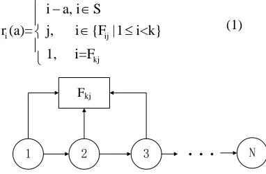
The system operation state is described as S= {1, 2…N}. State 1 means the system is “as good as new”. Each state gets closer to state N means higher deterioration degree. Meanwhile, the failure state is described as F= {Fij, |i∈ (1, 2,…, K), j∈S}.
Different state has different probabilities transfer to failure states. Thus the total state space is O=S∪F. Fig1 shows the deterioration process if no repair takes place of the model. De Leve [12] defined it as a natural process. If seperate major failure as an independent state, the state space of the model is same as Kim described [9].
2.2 Maintenance Action Space
Consider the system is in state i. Then the maintenance action “a” repairs the system from state i to state i-a. a=0 means no repair actions are taken, while a=i-1 means the action repairs the system to state 1 which means replacement actions are taken. Then the action space associate to operational space i is A(i)={ 0≤a≤i-1, a∈Z}. For any failure state Fij, a repair action Rij will be taken
to repair the system back to state j. Then, A(Fij)={Rij}. For state i, after repair action a has
been carried out, the repaired state will be:
i ij
kj
i a, i S
r (a)= j, i {F |1 i<k}
1, i=F
− ∈
∈ ≤
(1)
1 2 3 N
Fkj
[image:2.612.324.515.403.528.2]...
Figure 1. The System Deterioration Process Without Maintenance Action
2.3 Transition Probabilities
Based on the definitions above, if the system is in state i∈O, then action a∈A(i) is taken, the system will be repaired to state ri(a). We define
pij(a) as the probability that the system will be in
state j while the current state is i and an action a is taken. When no actions are taken, a=0, pij(a) =pij(0)
999
2.4 Expected Cost and Time between Epochs
Define u(i) as the time system will stay in state i if no action is taken. Define di as the cost per unit
time when system stays in state i. Define bi(a) as
the cost of state i with action a and ti(a) as time cost
of state i take action a. Obviously, if no action is taken, bi(a)=bi(0)=ti(0)=0. Define m as the system
cost with general repair. Then we can get the total cost of system in state i take action a is:
i i
i i i r (a ) r (a )
c (a)
=
b (a)
+
mt (a) d
+
u
(2)The total time stay in the interval is:
i
i
(n)
t (a)
iu
r (a )T
=
+
(3)3. COMPUTATIONAL APPROACH
The object of this model is to minimize the long run cost of the system per unit time. In some level, the cost of maintenance and system reliability is a pair of contradictions. Design more redundant equipment and backup system, full scale condition monitoring, frequent inspection, choose replacement rather than repair. All will highly increase systems reliability. However, in most cases, resources and time for maintenance are limited while as higher reliability as possible is requested. Thus, how to get optimal maintenance policy to use resources (manpower, time, money) efficiently becomes an important work.
Generally, there are several kinds of optimal maintenance works depend on the system kinds. A) The system is inspected periodically. Then the optimal time between inspections is an interesting work. The objection of the work is to find out the longest interval between inspections, while keep the system on a certain safety and reliability level. B) The system is under continuous monitoring. Then the determination of detailed maintenance action is an interesting and critical issue. When the system achieves a certain need-action state, repairing or replacement may both be able to bring the system to a better state. Repair cost less but can’t bring the system to the best state. And after more repairs, the system won’t be able to repair back to the ideal situation. Replacement cost more and makes the system brand new. It will restore the theoretically longest system remaining life. For long time consideration, what maintenance policy is the best is a considerable issue.
Define Z as policies set. Z includes all alternative policies. Define z∈Z as a function associated with state i. Generally, the optimization process of maintenance policy followed next steps [9]:
1) Choose a policy z∈Z.
2) Compute g, vi, i∈O as solution to linear
system equations:
i i i ij j j
v =c (z(i)) g (z(i)) p (z(i))v
O
T
∈
− +
∑
, i∈O, (4)
vo=0, for some v∈O
3) For each state i∈O, using the values g and vi
calculated in step 2), determine the action ai∈A(i)
minimizes the expression
i i i i ij i j
j
c (a ) g (a ) p (a )v
O
T
∈
− +
∑
(5)
The new policy z’∈Z is obtained by taking z’(i)=ai for each i∈O.
4) If z’=z, then the optimal stationary policy is z. Otherwise, return step 1) and replace z with z’.
As shown above, the general method is based on the idea that the minimum cost makes the best maintenance policy. This idea adopted well in many conditions. However, building up the model is different from using it in practical processes. For example, for a newly established system, the deterioration process, the transition probability, and failure transportation regularity are all unknown. There are several solutions to solve the problem:
1. Design rational experiments and trial operation of the system.
2. Analyze the detail deterioration process of the system.
3. Use condition monitoring and risk estimation techniques to manage the system life cycle.
In the next section, how the solution 3 influence the model will be further discussed.
4. CONDITION MONITORING
TECHNIQUE
1000 for the purpose of determining the current “health status” of a system’s internal components and predicting its remaining operating life. With the development of signal prediction technology and computer technology, continuous system state monitoring gradually steps from theory to practice. But how does it influence the traditional Markov deterioration model and how to count the condition monitoring and state prediction technology into optimal maintenance policy computation has not been properly discussed before.
The state space, maintenance action space, and transition probabilities wouldn’t change by the conditional monitoring and state prediction technology.
The model described in section 2 is already a model with continuous condition monitoring technology because the system states are precisely determined. If the model is based on interval inspection, the time of the decision making epoch would include interval between inspections.
5. RISK ESTIMATION
In MSS system, the estimation of system reliability and risk level can be considered in two ways:
1. Limited the system states to certain safety level. For each state, the system reliability and risk level can be settled. Then according to the required safety level, we can get the certain critical state. When the system state is worse than it, the action will have to be replacement or general repair. When the system state is better than it, the system will be surely above the required safety level. Thus, more consideration will put into calculate the optimal maintenance policy of the system states above the required safety level. The states space of the model would include states above the certain risk level.
2. For some complicate systems, analysis safety level and consequence of certain actions is a feasible way to describe system reliability and risk level. For computing the total cost of maintenance policy, risk and consequences should be finally calculated into the cost. Li and Gao’s [13] method to analyze risk and maintenance cost is a referential approach. Firstly, FMECA (Failure Mode, Effects and Criticality Analysis) are used to analyze important equipment’s failure mode analysis, failure cause analysis and failure consequence analysis. Secondly, high, medium criticality failures would be analyzed by FTA (Fault Tree analysis) to find the root causes of failures. Then use the matrix to evaluate the criticality in four aspects: safety,
environment, production loss, and maintenance cost. The expected cost of the model should include safety, environment and production loss.
The method 2 is adopted in this paper. Define Lij
as loss cost by Fij. Then equation in step 2 and 3 of
the computational approach would be
i i i ij j ij j
j j
v =c (z(i)) g (z(i)) p (z(i))v + p (z(i))
O F
T L
∈ ∈
− +
∑
∑
(6)i i i i ij i j ij i j
j j
c (a ) g (a ) p (a )v + p (a )
O F
T L
∈ ∈
− +
∑
∑
(7)The introduction of the last element of formular connected risk evaluation to total cost. With the participation of condition monitoring and state prediction, the real time dynamic optimal maintenance policy can apply to real production systems.
6. EXAMPLE AND DISCUSSION
In this section, a similar example as Kim [9] presented in 2009 is used. Define the system has 3 states and subject to 7 minor/major failures. Three kinds of maintenance policies are considered: do-nothing, repair and replacement. The total state space O= {1, 2, 3, F11, F21, F12, F22, F13, F23, F33}.
This example considers 3 operational states (1-3), 7 failure states (F11-F33) to describe multi-kinds
failure. Table1 provides the mean transition costs and times of the process. The natural evolution of the system is described by transition probability matrix (7)
0 0.1 0.2 0.1 0.2 0 0 0 0 0.4
0 0 0.1 0 0 0.1 0.2 0 0 0.5
0 0 0 0 0 0 0 0.1 0.2 0.7
0 0 0 1 0 0 0 0 0 0
0 0 0 0 1 0 0 0 0 0
=
0 0 0 0 0 1 0 0 0 0
0 0 0 0 0 0 1 0 0 0
0 0 0 0 0 0 0 1 0 0
0 0 0 0 0 0 0 0 1 0
0 0 0 0 0 0 0 0 0 1
P
(7)
The start initial policy is z0={0, 0, 0, R11, R21,
R12, R22, R13, R23, R} which no action is taken in
operational states. Using Eqs.described in section 3, the valve is obtained: v1=-8562.2, v2=-4159.4,
v3=1587.5, vF11=-7218.8, vF21=-6946.9, vF12
=-6275.0, vF22=-4803.1, vF13=-2831.2, vF23=-1359.4,
vF33=0, and g=106.6. After carrying out the
policy-improvement step described in Eq. (5), a new policy is obtained z1= {0, 1, 2, R11, R21, R12, R22,
R13, R23, R} ≠z0. Thus, return to step1 and define
1001 optimal maintenance policy is z= {0, 1, 2, R11, R21,
R12, R22, R13, R23, R} with the optimal cost rate
g=100.4.
Table 1. Expected Costs and Times
State 1 2 3 F11 F21 F12 F22 F13 F23 F33
ui 100 80 60 - - - -
di 10 15 20 - - - -
ti(1) - 20 30 - - - -
bi(1) - 4000 4500 - - - -
ti(2) - - 50 - - - -
bi(2) - - 8000 - - - -
ti(Rij) - - - 10 15 20 25 30 35 -
bi(Rij) - - - 3000 3500 4000 4500 5000 5500 -
ti(R) - - - 60
bi(R) - - - 9000
Lij - - - 500 800 1500 3000 5000 6500 8000
Tbale 2 Summary of Values and Policies Determined after Each Iterations
1 2 3 F11 F21 F12 F22 F13 F23 F34 g
z0 0 0 0 R11 R21 R12 R22 R13 R23 R
vi -8562 -4159 1587 -7219 -6947 -6275 -4803 -2831 -1359 0 106.6
z1 0 1 2 R11 R21 R12 R22 R13 R23 R
vi -7695 -3299 1292 -6529 -6225 -5522 -4019 -2016 -513 0 100.4
z2 0 1 2 R11 R21 R12 R22 R13 R23 R
Table 3. Expected Costs (102RMB) and Times (102h) for Main Pump
State 1 2 3 4 F11 F21 F12 F22 F13 F23 F24 F34
ui 110 82 65 37 - - - -
di 8 25 20 30 - - - -
ti(1) - 0.1 0.2 0.4 - - - -
bi(1) - 200 350 500 - - - -
ti(2) - - 0.5 0.8 - - - -
bi(2) - - 700 1000 - - - -
ti(3) - 1.5
bi(3) - 12000
ti(Rij) - - - - 0.02 0.03 0.05 0.08 0.5 0.6 0.8 -
bi(Rij) - - - - 150 210 300 500 700 720 810 -
ti(R) - - - 1.6
bi(R) - - - 18000
Lij - - - 80 180 350 620 1200 2100 3000 10000
Tbale 4 Summary of Values and Policies Determined after Each Iterations for Main Pump 1
(×
104)
2 (×
104)
3 (×
104)
4 (×
104)
F11
(×
104)
F21
(×
104)
F12
(×
104)
F22
(×
104)
F13
(×
104)
F23
(×
104)
F24
(×
104)
F34
(×
104)
g
z0 0 0 0 0 R11 R21 R12 R22 R13 R23 R24 R
vi -11.08 -7.10 -5.63 -2.67 -11.06 -11.04 -7.04 -6.99 -5.48 -5.39 -2.35 0 805.3
z1 0 1 2 3 R11 R21 R12 R22 R13 R23 R24 R
vi -3.95 -3.93 -4.22 -2.76 -3.93 -3.91 -3.87 -3.82 -4.04 -3.95 -2.40 0 245.3
z2 0 1 1 3 R11 R21 R12 R22 R13 R23 R24 R
-3.98 -3.96 -2.09 -2.78 -3.96 -3.94 -3.89 -3.85 -2.07 -2.06 -2.41 0 96.0
z3 0 1 1 3 R11 R21 R12 R22 R13 R23 R24 R
1002 In oil long distance transportation process, main pump is the heart of the system. Impeller of the pump suffered to corrosion, aging and fatigue etc. multi failure models.
Based on field experience and historical records, the main pump has 4 states and subject to 2 minor failures and 1 major failure. Four kinds of maintenance policies are considered: do-nothing, minor repair, major repair and replacement. The total state space O’= {1, 2, 3, 4, F11, F21, F12, F22,
F13, F23, F24, F34}. Table 3 provides the mean
transition costs and times of the process. The natural evolution of the system is described by transition probability matrix (8)
0 0.15 0.1 0.05 0.03 0.02 0 0 0 0 0 0.005
0 0 0.05 0.03 0 0 0.03 0.02 0 0 0 0.008
0 0 0 0.1 0 0 0 0 0.03 0.02 0 0.01
0 0 0 0 0 0 0 0 0 0 0.05 0.3
0 0 0 0 1 0 0 0 0 0 0 0
0 0 0 0 0 1 0 0 0 0 0 0
=
0 0 0 0 0 0 1 0 0 0 0 0
0 0 0 0 0 0 0 1 0 0 0 0
0 0 0 0 0 0 0 0 1 0 0 0
0 0 0 0 0 0 0 0 0 1 0 0
0 0 0 0 0 0 0 0 0 0 1 0
0 0 0 0 0 0 0 0 0 0 0 1
P
(8)
The start initial policy is z0={0, 0, 0, 0, R11, R21,
R12, R22, R13, R23, R24, R34, R} which no action is
taken in operational states. Using Eqs.described in section 3, the valve is obtained: v1=-11.08×10⁴,
v2=-7.10×10⁴, v3=-5.63×10⁴, vF11=-2.67×10⁴,
vF21=-11.06×10⁴, vF12=-11.04×10⁴, vF22=-7.04×
104, vF13=-6.99×10⁴, vF23=-5.48×10⁴, vF24=-5.39
×104, vF34=-2.35×10⁴,vF33=0, and g=805.3. After
carrying out the policy-improvement step described in Eq. (5), a new policy is obtained z1= {0, 1, 2, 3,
R11, R21, R12, R22, R13, R23, R24, R34, R} ≠z0.
Thus, return to step1 and define z1 as the initial policy. Policies obtained after each iteration are summarized in Table 2. After two steps of optimization, the final optimal maintenance policy is z= {0, 1, 1, 3, R11, R21, R12, R22, R13, R23, R24,
R34, R} with the optimal cost rate g=96.0.
8. CONCLUSIONS
This paper presented a mult-state model for a system subject to multi-failures. The deteriorating system was described by a semi-markov process. The objection was to find out the minimum long-run expected average cost per unit time. The model considered influence of condition monitoring system and risk evaluation. A numerical example was presented to certify the effect of the algorithm. The suggestion for future research is to consider the
influence of migration of failure states in the production system.
ACKNOWLEDGMENT
The authors would like to thanks to the colleges of Research Center of Oil & Gas Safety Engineering Technology for their incredible help and suggestions. The research is supported by National Science and Technology Major Project of China (Grant No. 2011ZX05055), National Key Technology Research and Development Program of China (Grant No. 2011BAK06B01) and National Natural Science Foundation of China (Grant No. 51005247).
REFRENCES:
[1] W.P. Pierskalla, J.A. Voelker, “A survey of maintenance models: the control and surveillance of deteriorating systems,” Naval
Research Logistics Quarterly, Vol. 23, No. 3,
Sep 1976, pp. 353-88.
[2] C. Valdez-Flores, R.M. Feldman, “A survey of preventive maintenance models for stochastically deteriorating single-unit systems,” Naval Research Logistics, Vol. 36, No. 4, Aug 1989, pp. 419-46.
[3] Y.S. Sherif, M.L. Smith, “Optimal
maintenance models for systems subject to failure: A Review,” Naval Research Logistics
Quarterly, Vol. 28, No. 1, Mar 1981, pp.
47-74.
[4] G. Levitin, A. Lisnianski, “Optimization of imperfect preventive maintenance for multi-state systems,” Reliability Engineering &
System Safety, Vol.67, No.2, Feb 2000, pp.
193–203.
[5] N. Nahas, A. Khatab, D.A. Kadi, M.
Nourelfath, “Extended great deluge algorithm for the imperfect preventive maintenance optimization of multi-state systems,”
Reliability Engineering & System Safety,
Vol.93, No.11, Nov 2008, pp.1658–1672. [6] J.H. Chiang, J. Yuan, “Optimal maintenance
policy for a Markovian system under periodic inspection,” Reliability Engineering & System
Safety, Vol.71, No.2, Feb 2001, pp.165-172.
[7] M.L. Neves, L.P. Santiago, C.A. Maia, “A condition-based maintenance policy and input parameters estimation for deteriorating systems under periodic inspection,” Computers &
Industrial Engineering, Vol.61, No.3, Oct 2011,
1003 [8] S. Wu, W. Wang, “Optimal inspection policy
for three-state systems monitored by control
charts,” Applied Mathematics and
Computation, Vol.217, No.23, Aug 2011,
pp.9810–9819.
[9] M.J. Kim, “Viliam Makis, Optimal
maintenance policy for a multi-state deteriorating system with two types of failures under general repair,” Computers & Industrial
Engineering, Vol.57, No.1, Aug 2009, pp.298–
303.
[10] S.J. Han, J.E. Yang, “A quantitative evaluation of reliability of passive systems within probabilistic safety assessment framework for VHTR,” Annals of Nuclear Energy, Vol.37, No.3, Mar 2010, pp.345–358.
[11] A. Veeramany, M.D. Pandey, “Reliability analysis of nuclear piping system using semi-Markov process model,” Annals of Nuclear
Energy, Vol.38, No.5, May. 2011, pp:1133–
1139.
[12] G.D. Leve, A. Federgruen, H.C. Tijms, “A general Markov decision method I: model and techniques,” Advances in Applied Probability, Vol.9, No.2, Jun 1977, pp.296–315,.
[13] D. Li, J. Gao, “Study and application of Reliability-centered Maintenance considering Radical Maintenance,” Journal of Loss
Prevention in the Process Industries, Vol.23,