Journal of Theoretical and Applied Information Technology
20th November 2014. Vol. 69 No.2© 2005 - 2014 JATIT & LLS. All rights reserved.
ISSN: 1992-8645 www.jatit.org E-ISSN: 1817-3195
375
ENERGY EFFICIENT RECLUSTERING ALGORITHM FOR
HETEROGENEOUS WIRELESS SENSOR NETWORKS
C.P. SUBHA1, Dr. S.MALARKKAN2
Research Scholar ,ECE Department, Sathyabama University, Chennai , India Professor &Principal, ManakulaVinayagar Institute Of Technology, Puducherry, India
E-mail: [email protected], [email protected]
ABSTRACT
Wireless sensor networks are composed of a large number of sensor nodes with limited energy resources. One critical issue in wireless sensor networks is how to gather sensed information in an energy efficient way since the energy is limited. The clustering algorithm is a technique used to reduce energy consumption. It can improve the scalability and lifetime of wireless sensor network. In this paper, we introduce an adaptive clustering protocol for wireless sensor networks, which is called Adaptive Decentralized Re-Clustering Heterogeneous Protocol (ADRHP) for Wireless Sensor Networks. In ADRHP, the cluster heads and next heads are elected based on residual energy of each node and the average energy of each cluster. Clustering has been well received as an effective way to reduce the energy consumption of a wireless sensor network. Clustering is defined as the process of choosing a set of wireless sensor nodes to be cluster heads for a given wireless sensor network. Therefore, data traffic generated at each sensor node can be sent via cluster heads to the base station. We introduce ADRHP, for electing cluster heads and next heads in wireless sensor networks. The selection of cluster heads and next heads are weighted by the remaining energy of sensor nodes and the average energy of each cluster. ADRHP is an adaptive clustering protocol; cluster heads rotate over time to balance the energy dissipation of sensor nodes.The simulation results show that ADRHP achieves longer lifetime and more data messages transmissions than current neural network based clustering protocols in wireless sensor networks.
Keywords: REBCS, ADRHP,RECLUSTERING.
1. INTRODUCTION
Wireless Sensor Networks (WSNs) are used as an emerging technology which holds the potential to revolutionize everyday life.The most important difference of Wireless Sensor Network (WSNs) with other wireless networks may be constraints of their resources, especially energy which usually arise from small size of sensor nodes. A sensor node basically consists of a microcontroller consumption. (processor and memory), sensors, analog-to-digital converter (ADC), transceiver (sender and receiver) and power supply. The provision of sensors is to gather information about the physical world, for instance, temperature, light, vibrations, and pressure. The individual sensor nodes are inherently resource constrained due to size limitation (form factor), price and power consumption.
2. SOM BASED ROUTING PROTOCOLS
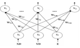
The Self-Organizing Map (SOM) is an unsupervised neural network structure consists of neurons organized on a regular low dimensional grid.
Each neuron is presented by an N-dimensional weight vector where n is equal to the dimensions of input vectors. Weight vectors (or synapses) connect the input layer to output layer which is called map or competitive layer. The neurons connect to each other with a neighbourhood relation as shown in Fig. 1. Every input vector activates a neuron in output layer (called winner neuron) based on its most similarity. The similarity is usually measured by Euclidian distance of two vectors,
2 n
1
i ij i
j
W
x
D
∑
=
−
376 Dj Close observations in input space would activate two close units of the SOM. The learning phase continues until the stabilization of weight vectors.
)
(
, . , ,
,
old j i i j i old j i new j
i
w
h
x
W
w
=
+
−
(2)Where xi is the input sample, Wi,jold is the previous weight vector between input vector xi and weight vector connected to output neuron j,hi,j is the neighbourhood function and Wi,jnew is the updated weight vector between input neuron i and output neuron j. There are different applications for SOM neural networks in WSNs routing protocols. These applications can be divided into three general groups: deciding optimal route, selection of cluster heads and clustering of nodes.
3.R-EBCS
In order to use the effectiveness of cluster-based routing algorithms in increasing of WSNs lifetime, Energy Based Clustering Self organizing map (R-EBCS) is used. The classic idea for topological clustering and incorporate a topology-energy based clustering method in order to
Fig.1 SOM Topology
approach to our main goal in WSNs, extending life time of the network with enough network coverage. In our idea, energy based clustering can create clusters with equivalent energy levels. In this way, energy consumption would be better balanced in whole network.
The operation of the algorithm is divided into rounds in a similar way to LEACH-C. Each
round begins with a cluster setup phase, in which cluster organization takes place, followed by a data transmission phase, throughout which data from the simple nodes is transferred to the cluster heads. Each cluster head aggregates/fuses the data received from other nodes within its cluster and relays the packet to the base station. In every cluster setup phase, Base Station has to cluster the nodes and assign appropriate roles to them. After determining the cluster heads of current round, BS sends a message containing cluster head ID for each node. If a node's cluster head ID matches its own, the node is a cluster head otherwise it is a normal node.
3.2 Cluster Setup Phase
The protocol uses a two phase clustering method SOM followed by K means algorithm which had been proposed in with an exact comparison between the results of direct clustering of data and clustering of the prototype vectors of the SOM[1]. We selected SOM for clustering because it is able to reduce dimensions of multi-dimensional input data and visualize the clusters into a map. In our application, dimensions of input data relates to the number of variables (parameters) that we need to consider for clustering. The reason for using SOM as preliminary phase is to make use of data pre-treatment (dimension reduction, regrouping, visualization) gained by SOM. Therefore the data set is first clustered using the SOM, and then, the SOM is clustered by k means. The variables that we want to consider as SOM input dataset is x and y coordination of every node in network space and the energy level of them. So we will have a D matrix with N-3 dimensions. Since we are applying two different type variables, first we have to normalize all values.
)
min
(max
min
'
a a
a
−
−
=
ν
V
(3)3.1 Algorithm Assumptions
The proposed algorithm (REBCS) is more like LEACH-C and LEA2C protocols. Thus the assumption about BS cluster formation tasks and energy consumptions models of normal and cluster head nodes are the same as previous.
So by means of above equation, our dataset matrix would be:
=
max max
1
max
max 1
max 1
max 1
. .
E E yd
yd xd
xd
E E yd
yd xd
xd
D
n n
(4)
377 YD=(ydl. ..ydn) are Y coordinates, E=(El ...En) are energy levels of all sensor nodes of the networks, xdmax is the maximum value for x coordinate of the network space, ydmax is the maximum value for Y coordinate of network space and Emax is the remain energy of maximum energy node of the network( at the beginning it is equal to E initial).In order to determine weight matrix, Base Station has to select m nodes with highest energy in the network. At the beginning, the nodes have equal energy level according to our assumptions. So we can partition the network space to m regions and select the nearest node to center of every region. However due to using two phase SOM-K means method, we usually need to consider a rather large value for m, especially in large WSNs. In this case we can choose the m nodes randomly. We need three variables of these selected (high energy) nodes to apply them as weight vectors of our SOM: their x coordinate, their y coordinate and their energy level. Therefore our weight matrix would be,
− − = max m max 1 max m max 1 max m max 1 E E E E yd yd yd yd xd xd xd xd W 1
1 L L
L L L
L L
L (5)
[image:3.595.118.258.564.648.2]W is the weight matrix of SOM, XD= (xd1..xdn) are x coordinates, YD= (yd1…ydn) are y coordinates and (1-E1/Emax…1-En/Emax) are consumed energy of m selected max energy sensor nodes. In this way we want to move the nodes with less energy towards max energy nodes in order to form balanced clusters. So the SOM topology structure would be as Fig. 2.
Fig. 2 SOM topology structure
In our application, learning is done by minimization of Euclidian distance between input samples and the map prototypes weighted by a neighbourhood function h i,j.So the criterion to be
minimized is defined by,
∑ ∑
= = −=
N 1 K M 1j jNX w x
SOM 2 k j K
h
N
1
E
) ( . ) ( ( , (6)Where N is the number of data samples, M is the, number of map units; N(x k)is the neuron having the closest referent to data sample N(xk)and his the Gaussian neighbourhood function defined by:
− = − t 2 2 j j 2 r r exp t j i h σ ) (
. (7)
Where
2 j j
r
r
−
the distance between map unit jand input sample i and t σ is the neighbourhood radius at time t which is defined by:
)
(
)
(
T
t
exp
t
=
σ
o−
σ
(8)Where t is the number of iteration, t is the maximum number of iteration or the training length. The distance between X k and weight vectors of all map neurons are computed. A neuronN(Xk) which has the minimum distance with input sample X k , would win the competition phase: 2 K J m j 1
K
arg
min
W
X
X
N
=
<≤ .−
)
(
(9)The neighbourhood radius is a great value at the beginning and it will reduce with increasing of the time of the algorithm in every iteration. After competition phase, SOM should update the weight vector of the winner N(Xk)and all its neighbours which placed at the neighbourhood radius of (R N(Xk)).
)) ( ) ( ( ) ( ) ( ) ( ) 1 ( . , ( ) .
. t w h t x t W t w j k k x N j j
j + = + k −
t t α Else,
)
(
)
1
(
. .t
w
t
W
jj
+
=
(10)Where hj,n(x(k)(x(t) is the neighborhood function attimet and a ( t ) is the linear learning factor at
378
)
1
(
)
(
t
t
T
0
−
=
α
α
(11)Where 0 is the initial learning rate, t is the number of iteration and T is the maximum training length. The learning phase repeats until stabilization (no more change) of weight vectors. SOM clusters n data samples into m map units (clusters). Now the SOM should be given to K means algorithm as input. K-means, partitions the data set into K subsets (clusters) such that all objects in a given dataset are closest to the same centroid. K-means randomly selects K of objects as cluster centroids. Then other objects are assigned to these clusters based on minimum Euclidean distance to their centroids. The mean of every cluster is recomputed as new centroids and the operation will continue until the cluster centers do not change anymore. The criterion to be minimized in K-means is defined by:
2 c
l k x Q
k means K K
C
x
c
1
E
∑ ∑
= ∈
−
=
−
(12)Where C is the number of clusters, Q kis Kth cluster, Cks the centroid of cluster Qk.The best value for K (optimal number of clusters) can be determined with an index. We selected Davies-Bouldin index. DB index actually compute the ratio of intraclusters dispersion to inter-cluster distances by:
∑
=
+
=
C 1K ce k l
l c k c DB
Q
Q
d
Q
S
Q
S
max
C
1
I
)
,
(
)
(
)
(
(13) k i 2 k i k cQ
c
x
Q
s
∑
−
=
)
(
(14)2
l k l k
cl
Q
Q
c
c
d
(
,
)
=
−
(15)Where C is the number of clusters, Scis the intra cluster dispersion and dcl is the distance between centroids of two clusters k and l. Small values of DB index correspond to clusters which are compact, and whose centers well separated from each other. Consequently, the number of clusters that minimizes DB index is taken as the optimal number of clusters. Now, Base station knows the optimal number of clusters and their member nodes. So the next step before going to transmission phase is selection of suitable cluster heads for each
cluster and assigning appropriate roles to each node.
3.3 Cluster Head Selection Phase
Different parameters can be considered for selecting a CH in a formed cluster. In three criterions have been considered for CH selection:
1. The sensor having the maximum residual energy
level
2.The nearest sensor to the BS
3. The nearest sensor to gravity center (centroid) of the cluster.
When we select the nearest node to BS in a cluster as CH, we insure to consume least energy to transmit the messages to BS. Also the nearest sensor to gravity center (centroid) of the cluster insures least average energy consumption for intra cluster communications. Whereas, selecting nodes with maximum residual energy shows better results compared to the nearest node to base station and nearest node to centroid level.
3.4 Transmission Phase
After formation of clusters and selecting their related cluster heads now it's time to send data packets sensed at normal nodes to their related cluster heads and after applying data aggregation functions to received packets by CHs, send messages on to the base station. The energy consumption of all nodes is computed.
)
,
(
)
,
(
k
d
E
()E
k
d
E
amp Tx l Tx
Tx
=
+
− (16) ∈ + < ∈ + = − − else d d if crossover , . . ) , ( . , . ) , ( . ) , ( 4 amp ray two elec 2 friss elec Tx d k d k E k d k d k E k d k
E (17)
The energy consumption for receiving k bits of data is computed by:
elec else
Rx
Rx
k
d
E
k
k
E
E
(
,
)
=
(
)
=
.
379 Where Eelec is the energy of electronic transmission/reception, kis the size of message in bit, dis the distance between transmitter and receiver, E tx_amp is amplification energy, friss ε is amplification factor, d crossover is a threshold distance in which transmission factors change. Also energy consumption of data aggregation of CHs is:
msg
bit
NJ
E
DA=
5
/
/
(19)After every transmission phase, we count a new round and would have a cluster head rotation (in the case of using maximum energy criterion) The best time for re-clustering can be when a relative reduction occurs in energy level of nodes. So the energy level of m selected highest energy nodes are checked regularly. 20 percent depletion of initial energy for first time re-clustering phase and 5 percent depletion for next times are used. When the clustering threshold is satisfied, BS sends a re-clustering message to whole network.
2.Cluster set-up phase:
a. Clustering of WSN through SOM and K-mean clustering method by using sensor coordinates and remained energy as SOM inputs and selecting of m nodes with maximum energy level as the weights of SOM map units. The value for m can be different for every scene and experimental. b. selection of cluster heads for every cluster with one of the 3 criteria mentioned (maximum energy sensor, nearest sensor to BS and nearest sensor to gravity center of the cluster).
c. assigning roles to every node (CH or Normal
node) by BS.
3.Data transmission phase:
a. Data transmission from normal nodes to CHs. Energy consumption of nodes is then computed using energy mode.
b. Data aggregation and or fusion of received packets and sending results to BS by CHs. energy consumption of CHs is then computed.
c. CH selection if the CHs had been chosen according to maximum energy criteria
d. Repeat the steps 3.a to 3-d until the average energy level of m selected maximum energy nodes show a 20 percent reduction for first time re clustering and 5 percent for next times.
4.Repeat the steps 2 to 3 until all sensors in the network die.
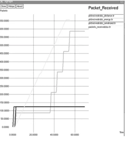
Packet received ratio: The packet received ratio is defined as the ratio of number of packets received to the total number of packets sent. Here the packet delivery ratio is more in cluster head selection using Residual energy method compared to other two methods that is Centroid method and nearest to base station method.
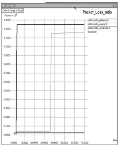
Packet loss ratio: The packet loss ratio is average in the case of residual energy based cluster head selection but more in centroid method. Hence, in distance method the packet loss will be less compared to other two methods (energy method and centroid method).
So, we can summarize the algorithm into following Steps:
1.Initialization:
Random deployment of N Homogeneous sensors in a given space and with the same energy level.
Residual energy: The residual energy method is the amount of remaining energy left after cluster head formation. In the energy method the nodes are alive for long period than in cluster head selection using Centroid method and Nearest to base station method.
4. ADRHP
ADRHP (Adaptive Decentralized Re-clustering Heterogeneous Protocol) is a Re-clustering protocol for wireless sensor networks. It is used to
380
Fig.3 ADRP operations
The wireless sensor network consists of N sensor nodes, and sensor nodes are deployed randomly in the sensing field. As shown in Fig. 2, the base station splits the network into clusters and elects some sensor nodes as cluster heads, which collect sensor data from other nodes in the clusters and transfer the aggregated data to the base station.
Fig.4 clustering topology
Each cluster has one cluster head, next heads and set of sensor nodes. Since data transfers to the base station dissipate much energy, the nodes take turns with the transmission by rotating the cluster heads, which leads to balanced energy consumption of all nodes and hence to a longer lifetime of the network. In this proposed protocol, we consider the following assumptions:
1. There is a base station located far away from the square sensing field.
2. Each sensor node is assigned a unique identifier (ID)
3. Each sensor node has power control and the ability to transmit data to any other sensor node or directly to the base station.
4. Nodes are immobile.
5. All the sensor nodes are location aware. To get the information, sensor nodes can use GPS or other location detect scheme
4.1 ADRHP Algorithm
A. Initial Phase
During the initial phase, Base station receives information about current locations and remaining energy levels from sensor nodes. The base station uses the remaining energy level and locations to split the network into clusters and determine the cluster heads. Once the clusters are formed, the base station determines the next heads. In order to do this, the base station computes the average energy for each cluster in the network, and sensor nodes that have energy storage below this average cannot become next heads for this round. Once the cluster heads and next heads are determined, the base station broadcast the information including cluster heads and next heads to all sensor nodes. The initial phase consists of three stages: partition stage, selection stage and advertisement stage.
1.Partition stage
During this stage, each sensor node transmits the data of its position and the amount of energy to the base station. The sensor nodes get their current location by using a global positioning system receiver that is activated at the beginning of each initial phase. On receiving the data, the base station calculates the energy value of all sensor nodes and then elects the cluster heads by minimizing the total sum of the distances between the cluster heads and sensor nodes. Furthermore, base station makes sure that only nodes with enough energy are participating in the cluster heads selection. ADRHP can distribute the energy between the sensor nodes by positioning cluster heads into the centre of clusters. At end of this stage, ADRHP partitions the nodes into set of clusters and each cluster is managed by a selected cluster head. There are three different kinds of sensors: Cluster head, Sensor node and Next head Cluster head (super node)
Next head (advanced node)
Member node (normal node)
381 formed with the three types of nodes i.e, nomal nodes, advanced nodes and super nodes.
2. Selection stage
Cluster head is responsible for receiving all the data from nodes within the cluster, aggregating this data and send the aggregate data to the base station. If this role was fixed, the cluster head would quickly drain its limited energy and die. Therefore, ADRHP includes rotation of this role among all the sensor nodes in the network to distribute the energy load. In this stage, ADRHP protocol requires a set of sensor nodes to be elected as next heads. Once the clusters have been formed, the ADRP selects a set of sensor nodes as next heads. To do this, the ADRP computes the threshold (average energy) for each cluster, and whichever nodes have energy above this threshold can be next heads for the current round.
The ADRP repeats the following two steps for each cluster to select set of sensor nodes as next heads. ADRP computes the threshold for each cluster j.
∑
=
=
m
i j
Ei
t
m
T
1
)
(
1
. ( 20)
Where m is number of sensor nodes in cluster j. Ei(t)is the current energy of node i. The sensor nodes with higher energy are more likely to become next heads. If current energy of nodei greater than or equal toTj,the threshold of cluster j, the n node i is member of set NH j.
j j
i
NH
T
t
Ei
≥
∈
,
)
(
. (21)
Where NH j is the set of nodes that are eligible to be next heads in cluster j. Once NH j sets have been created, the ADRHP elects group of next heads from the sets and specifies its member nodes. At end of this stage, there are three different kinds of sensors:
1. Cluster heads collect sensor data from cluster members, aggregate the data and forward it to the base station.
2. Sensor nodes gather sensor data and forward the data to the cluster head.
3. Next heads act as sensor nodes but during the re-cluster stage each sensor node selects next head as new cluster head and switch to it.
3. Advertisement stage
During this stage, the base station sends a message containing the cluster head ID and next heads for each sensor node. If a node’s cluster head ID matches its own ID, the node is a cluster head; otherwise, the node is a sensor node.
B. Cycle Phase
During the cycle phase, each cluster head creates and distributes the TDMA schedule, which specifies the time slots allocated for each member of the cluster. The cluster head advertises the schedule to its cluster members through broadcasting. Each node is assigned a unique time slot during which it can transmit its data to the cluster head. Upon receiving data packets from its cluster nodes, the cluster head aggregates the data before sending them to the base station. At end of this phase each node selects next head as new cluster head and switch to it. The advanced nodes become the next cluster head. The nodes join the next cluster head and become cluster members in order to complete clusters forming. The cycle phase consists of three stages: Schedule stage, Transmission stage and Re-cluster stage.
1. Schedule stage
Once clusters have been formed, the sensor nodes must send their data to the cluster head. ADRHP uses TDMA, which allows the sensor nodes to enter a sleep mode when they are not transmitting data to the cluster head. Also, using a TDMA approach in intra cluster communication ensures there are no collisions of data within the cluster. Based on the number of nodes in the cluster, the cluster head node creates a TDMA schedule telling each node when it can transmit. The TDMA schedule divides time into a set of slots, the number of slots being equal to the number of nodes in the cluster. Each node is assigned a unique time slot during which it can transmit its data to the cluster head.
2. Transmission stage
The data transmission stage consists of three major activities:
382 •Data aggregation.
•Data sending.
At each sensing period, all sensor nodes send their data to their cluster heads and check the contents of incoming data and then combine them by eliminating redundant data. Then, the cluster heads transmit the aggregated data to the base station using a CSMA MAC protocol. The data aggregation is to minimize traffic load by eliminating redundancy.
3. Re-Cluster Stage
The ADRHP periodically re-clusters the network in order to distribute the energy consumption among all sensor nodes in a wireless sensor network. In the initial phase the base station sends messages containing the cluster head ID and next heads for each sensor node in the network. So, the sensor nodes can switch directly to the next heads without communicate with the base station. Thus, the ADRP protocol forms new clusters each cycle phase
5. SIMULATION RESULTS
Table1: Simulation Parameters
Type REBCS ADRHP
Channel Wireless channel
Wireless channel Radio
Propagation model
Propagation /Two ray ground
Propagation
/Two ray
ground Network
Interface type
Phy/Wireless Phy
Phy/Wireless Phy
Mac type MAC 802.11 MAC 802.11 Link layer
type
LL LL
Antenna Omni Omni
Max packets
50 50
Routing Protocol
AODV DSDV
Interface Queue type
Queue/Drop tail/PriQueue
Queue/ Drop tail/PriQueue Size of NW 500*500 500*500
No of
nodes
25 25
Simulation time
70min 70min
5.1 Simulation set up for REBCS and ADRHP
The simulation is done in NS2 Software. We evaluate our REBCS AND ADRHP algorithm using NS2. We consider a random network deployed in an area of 500*500The list of parameters are the radio propagation mode is Two Ray Ground, the channel type is wireless channel, antenna type is Omni antenna, maximum number of packet is 50, number of nodes used are 25, routing protocol is AODV in REBCS and DSDV in ADRHP, the interface queue type is Drop Tail, the network interface type is phy/wireless , the MAC type is 802-11.The sink is assumed to be situated 100metres away from the above specified area. The initial energy of all the nodes is assumed as 5 joules. The simulation time is 70 minutes.
[image:8.595.307.510.347.577.2]5.2 Simulation Results
Fig.6 Number of packets delivered
5.3 Throughput
383 ADRHP protocol compared to REBCS protocol as shown in fig.6.
[image:9.595.305.506.152.384.2]5.4 Packet loss
Fig 7 shows the Number of packets lost in REBCS algorithm for 3 cluster head selection methods i.e cluster head selected based on nearest to base station, residual energy and centroid method and packets delivered in ADHRP algorithm .
.Fig. 7Number of packet lost
It is found that the no of packets lost is less or negligible in the case of ADRHP compared to REBCS.
5. No of Nodes Vs Rounds
.
Fig.8 Alive sensor nodes versus rounds
In fig.8 the full node death occurs after 100 rounds in case of ADRHP protocol whereas in REBCS the full node dies within 75 rounds in case of all three types of cluster head selection. Simulated results shows that proposed protocol ADRHP has extended the lifetime of the network and has reduced the communication overhead compared to REBCS.
CONCLUSION:
[image:9.595.92.294.247.494.2]384
REFERENCES
[1] Xu Y, Heidemann J, Estrin D. Geography informed Energy Conservation for Ad-hoc Routing. In: Proc. 7th Annual ACM/IEEE Int’l. Conf. Mobile Comp and Net, 2001, pp. 70–84.
[2] Ye M, Li C. F, Chen G. H, Wu J. EECS: An Energy Efficient Clustering Scheme in Wireless Sensor Networks. In: Proceedings of IEEE Int’l Performance
Computing and Communications
Conference (IPCCC), 2005, p. 535-540.
[3] Yu Y, Estrin D, Govindan R.
Geographical and Energy-Aware Routing: A Recursive Data Dissemination Protocol for Wireless Sensor Networks. In: UCLA Comp. Sci. Dept. tech. rep., UCLA-CSD TR-010023(2001) .
[4] Yun S.U, Youk Y.S, Kim S.H, Study on Applicability of Self-Organizing Maps to Sensor Network. In: International Symposium on Advanced Intelligent Systems, Sokcho, Korea, 2007.
[5] Pottie G, Kaiser W, Wireless Integrated Network Sensors. In: Communication of ACM, Vol. 43, N. 5, pp. 51-58, May 2000.
[6] Raghunathan V, Schurghers C, Park S, Srivastava M. Energy-aware Wireless Microsensor Networks. In: IEEE Signal Processing Magazine, March 2002, pp. 4050.
[7] Shahbazi H, Araghizadeh M.A, Dalvi M. Minimum Power Intelligent Routing In Wireless Sensors Networks Using Self Organizing Neural Networks. In: IEEE
International Symposium on
Telecommunications, 2008, p. 354–358 .
[8] Vesanto J, Alhoniemi E. Clustering of Self Organizing Map. In: IEEE Transactions on Neural Networks, Vol. 11, No. 3, 2000, pp. 586-600.
[9] Vesanto J, Himberg J, Alhoniemi E, Parhankangas J. Self-Organizing Map in
MATLAB: The SOM toolbox. In: Proc of MATLAB DSP Conference, Finland, 1999, p.35-40 .
[10] Visalakshi N. K, Thangavel K. Impact of Normalization in Distributed K-Means Clustering. In: International Journal of Soft Computing 4, Medwell journal, 2009, p. 168-172
[11] Wei D, Kaplan SH, Chan H.A. Energy Efficient Clustering Algorithms for Wireless Sensor Networks. In: IEEE
Communication Society workshop
proceeding, 2008.
[12] Al-karaki J.N, Kamal A.E. Routing Techniques in Wireless Sensor Networks: A Survey, IEEE Wireless Communication, 2004, p.6-28
[13] Anastasi G, Conti M, Passarella A. Energy Conservation in Wireless Sensor Networks: a survey. In: Ad Hoc Networks, volume 7, Issue 3, Elsevier; 2009, p.537-568
[14] Aslam N, Philips W, Robertson W, Siva Kumar SH. A multi-criterion optimization technique for energy efficient cluster formation in Wireless Sensor networks. In: Information Fusion, Elsevier; 2010 [15] Sudhir G. Akojwar, Rajendra M. Patrikar
Improving Life Time of Wireless Sensor Networks Using Neural Network Based
Classification Techniques With
Cooperative Routing, international journal of communications, Volume 2, 2008. [16] C.P. Subha, Dr. S. Malarkan,
K.Vaithinathan, A Survey On Energy Efficient Neural Network Based Clustering Models In Wireless Sensor Networks,IEEE Transaction on Wireless sensor network,2013.