STABILITY ANALYSIS AND PARAMETER DESIGN OF
BLDC DRIVE UTILIZING ROOT-LOCUS APPROACH
1
M MURUGAN, 2R JEYABHARATH, 2P VEENA
1Assistant Professor, Department of Electrical and Electronics Engineering, K.S.Rangasamy College of
Technology, Tiruchengode, Tamilnadu, India.
2
Professor, Department of Electrical and Electronics Engineering, K.S.R Institute for Engineering and Technology, Tiruchengode, Tamilnadu, India.
E-mail: [email protected], [email protected]
ABSTRACT
The demands for BLDC motor drives in industrial applications are rapidly increasing due to its high efficiency, high power factor and lower maintenance. Therefore, it is necessary to design a stable control system for BLDC drive system to achieve a quality performance. The stability is a major problem in the closed loop BLDC drive system which may cause oscillations of constant or changing amplitude. This paper spotlights the movements of characteristic roots of the drive system on s-plane with the variation of system parameter gain ‘k’. The root locus and root contours of the BLDC drive system are portrayed in this paper which focuses the complete dynamic response of the system. Finally, the steady-state performance of the BLDC drive system has been investigated by calculating its steady-state error to various standard test signals. These analyses help a designer to easily visualize the effects of varying various system parameters on root locations. These analyses give good potential design specifications for the control engineers. The Matlab software package is used to analyze the results.
Keywords: Brushless DC (BLDC) Motor Drives, Root Locus, Root Contour; Parameter Design, Stability,
Steady-State Error.
1. INTRODUCTION
Now a day’s Brushless DC (BLDC) motors are becoming more popular due to high efficiency and lesser maintenance which will replace those inefficient motors. There are several inherent advantages in the Brushless PM motor drives, over other machine types. Most prominent among them are, they require lesser maintenance due to the elimination of the mechanical commutator and brushes. They also have high efficiency and high power density due to the absence of field windings. Applications of Brushless PM motor drives range from low speed such as servo position control to high speed such as in disk drives, electric vehicles and aerospace applications
A novel digital PWM controller was presented for a BLDC motor in [1] which treats the motor as a digital system. The characteristic equation of BLDC machine has been used to derive the design procedure, which involves simple first order non-homogeneous differential equations. The mathematical model of the BLDC motor is
presented in [4]. The operation of the hysteresis and PWM current controllers and the structure of the drive system are outlined in this paper. The development, design, and construction of a variable speed synchronous motor drive system were explained in [3]. In this paper, a current controller and speed controller was designed and an accurate prediction of the system behavior was obtained with the help of digital simulation. R.Krishnan etal [10] presented the design of current and speed controller for the PM Synchronous motor drive system. This design of speed controller has significant importance in the transient study and steady-state characteristics of the PMSM drive. The investigators have not analyzed the movement of the characteristic roots on the s-plane by varying the system parameters.
In this paper, the basic characteristic of the transient response of a closed-loop BLDC drive system is determined from the open-loop poles. The roots of the characteristic equation are plotted for all values of system gain parameter ‘k’ using root-locus method. Also, the root contour of the BLDC
ISSN: 1992-8645 www.jatit.org E-ISSN: 1817-3195
and ‘β’ are varied from zero to infinity. For the
closed-loop system presented in this paper, characteristic equation of a BLDC machine have been used to derive the design procedure. Finally, the steady-state performance of the BLDC drive system has been investigated by the steady- state error due to step, ramp and acceleration inputs. This helps to modify the open-loop poles and zeros of the drive system to meet the desired system performance specifications.
2. BRUSHLESS DC MOTOR DRIVE STRATEGIES
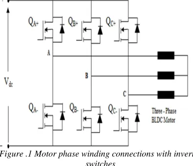
The most common topology used for a three-phase BLDC motor is MOSFET or IGBT three-phase inverter bridge. Figure 1 shows the connection of motor phase winding with the inverter switches. The windings employed in this type of motor are the same as those used in ordinary three-phase AC motors. The Hall sensor signals and back E.M.F variation of a three-phase BLDC motor are shown in Figure 2. The current is fed to the windings of the motor during the flat position of the back E.M.F waveform to achieve the constant output power and constant output torque respectively. Figure.2 demonstrates that the back E.M.F induced per phase of the motor winding is
constant for 1200 period. The commutation of a
[image:2.612.318.524.130.397.2]BLDC motor is controlled using solid state commutation [1].
Figure .1 Motor phase winding connections with inverter switches
The stator windings of the motor should be energized in a proper sequence for the rotation of the BLDC motor. Therefore, it is important to know the rotor position in order to follow the proper energizing sequence. The rotor position is sensed using Hall effect sensors which are embedded in the stator. Every 60 electrical degrees of rotation, one of the Hall sensors changes the state [11],[12]. R.krishnan derived the mathematical model for the BLDC drive system shown in Figure 1. In this
[image:2.612.92.289.448.617.2]paper, this model has been used for further analyzes of the performance of the BLDC drive system employing root locus technique.
Figure 2 Back E.M.F Variation with Rotor Electrical Angle
3. SPEED CONTROLLER OF THE BLDC DRIVE SYSTEM
The design of speed controller for a BLDC motor drive is important to judge the transient and steady-state characteristics of the drive system. The block diagram of the speed-controlled BLDCM drive is shown in Figure 3. The mathematical model of BLDCM drive mainly consists of two loops. One is the inner loop called current loop and the other is the outer loop called speed loop [6],[10].
The transfer function of PI controller is given by,
Gs ౩౩ ౩ (1)
The inverter is modeled by the following transfer function,
Gs
(2)
Where, K 0.65ౚౙ
ౙౣ
(3)
T
ౙ (4)
Where,
Vdc is the dc-link voltage input to the inverter,
Vcm is the maximum control voltage,
fc is the carrier frequency of the inverter.
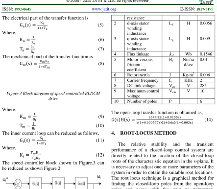
The electrical part of the transfer function is
Gs (5)
Where,
K
౩
(6)
T౧౩ (7)
The mechanical part of the transfer function is
[image:3.612.86.529.63.449.2]Gs ౣౣ౪ (8)
Figure 3 Block diagram of speed controlled BLDCM drive
Where,
K౪ (9)
T౪ (10)
The inner current loop can be reduced as follows,
Gs
(11)
Where,
K ౣ
మౘ (12)
The speed controller block shown in Figure.3 can be reduced as shown Figure 2.
Figure.4 Canonical form of speed controller block diagram
The forward path transfer function is given by,
Gs GsGsGs (13) The feedback path transfer function is given by,
Hs Gs (14)
The open-loop transfer function is given by,
GsHs
K
ୱK୧K୫K୲Hன
Tୱ 1 sTୱ
T୧T୫Tனsସ TனT୫ T୧Tன T୧T୫sଷ T୫ T୧ Tனsଶ s (15)
The BLDC drive system parameters are shown in Table.1
Table 1. BLDC drive parameters.
SL. NO
Parameter Symb
ol
Unit
Value
1 Stator winding Rs Ω 1.4
resistance
2 d-axis stator
winding inductance
Ld H 0.0056
3 q-axis stator
winding inductance
Lq H 0.009
4 Flux linkage af Wb 0.1546
5 Motor viscous
friction coefficient
Bt Nm/ra
d/sec 0.01
6 Rotor inertia J Kg-m2 0.006
7 Carrier frequency fc KHz 2
8 DC link voltage Vdc V 285
9 Maximum control
voltage
Vcm V 10
10 Number of poles P 6
The open-loop transfer function is obtained as,
GsHs &.&&&%!!&. &.&& !".$%&.&%% (14)
4. ROOT-LOCUS METHOD
The relative stability and the transient performance of a closed-loop control system are directly related to the location of the closed-loop roots of the characteristic equation in the s-plane. It is necessary to adjust one or more parameters of the system in order to obtain the suitable root locations. The root locus technique is a graphical method for finding the closed-loop poles from the open-loop poles and zeros with the gain as parameter. Therefore, root-locus method is used to obtain the qualitative information of stability and performance of the BLDC drive system [8],[9].
The open-loop transfer function of the speed controller system is obtained as,
GsHs !$. . !%&&' ".% (15)
The characteristic equation is given by
sସ
2233.267sଷ
869520.07sଶ
144328s k
ISSN: 1992-8645 www.jatit.org E-ISSN: 1817-3195
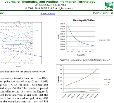
Figure 5 Root-locus plot for the speed control system
For the open-loop transfer function G(s) H(s),
the open-loop poles are located at s1=0; s2= -1.667;
s3=-500 and s4= -1731.6 for k=0. The open-loop
zero is located at s5= -64.516. The root-locus plot of
the speed controller system is shown in Figure 5. From the root-locus analysis, it can seen that the
root locus starts from the open-loop pole at s3=-500
and ends on the open-loop zero at s5= -64.516
when the gain is varied from zero to ∞. Another
root-locus starts at s4= 1731.6 is moved towards
-∞. They are on the negative real axis far away from
the dominant root locus which starts at s2=-1.667
and s1=0. Therefore s3, s4 and s5 have no significant
effect on the system performance.
Using Routh Array one can find that the system
is stable upto k=7.561×10¹¹.When k= 7.561×10¹¹
the natural frequency ωn of the system is
0.999rad/sec. For various values of damping factor the value of gain is obtained and portrayed as shown in Figure 6. The variation of overshoot, damped frequency and settling time versus gain ‘k’ are plotted as shown in Figure.6. Figure 7 demonstrates that when the damping ratio is increased the overall gain of the system is reduced. From the Figure7 it can be seen that when the gain ‘k’ is increased the percentage overshoot and damped frequency of the system is increased. Also,
when gain k=1.4×10⁸, the settling time is obtained
as ts=29ms. When k is increased to 1.6×10⁸, the
[image:4.612.135.525.36.390.2]settling time is reduced to 24ms and further increase in gain leads to increase in the settling time of the system.
[image:4.612.323.522.46.426.2]Figure.6 Variation of gain with damping factor
Figure 7 Variation of overshoot, damped frequency and settling time with gain
5. PARAMETER DESIGN BY THE ROOT CONTOUR METHOD
In many applications, the effects on the closed-loop poles need to be investigated when the system parameters other than the gain ‘K’ are varied. Using root-locus method the effects of other parameters can be easily investigated. This method of parameter design uses root-locus approach to select the values of the parameters and is called root contours [9], [13].
The characteristic equation of BLDC drive system is given by,
T୧T୫TனS ସ
TனT୫ T୧Tன T୧T୫S
ଷ
T୫ T୧ TனS
ଶ
1 KୱK୧K୫K୲HனS
౩ౣ౪ୌಡ
౩ 0
(17) S" ౣ ಡ S
$
ಡ
ౣಡ
ౣ S
౩ౣ౪(ಡ
ౣಡ S
౩ౣ౪(ಡ
౩ౣಡ 0
(18)
Let α ౩ౣ౪(ಡ
౩ౣಡ and
β ౩ౣ౪(ಡ
ౣಡ
-200 -150 -100 -50 0 50
-1500 -1000 -500 0 500 1000 1500 0.03 0.048 0.068 0.1 0.14 0.22 0.4 200 400 600 800 1e+003 1.2e+003 1.4e+003 200 400 600 800 1e+003 1.2e+003 1.4e+003 0.014 0.03 0.048 0.068 0.1 0.14 0.22 0.4 0.014 Root Locus
Real Axis (seconds-1)
i.e; ) *
+
(19)
Then the characteristic equation becomes,
Sସ ଵ
ଵ
ౣ
ଵ
ಡ S
ଷ ଵ
ಡ
ଵ
ౣಡ
ଵ
ౣ S
ଶ
βS α 0 (20)
Sସ
2215.267Sଷ
869520.2017Sଶ
βS α 0
(21)
This is a fourth order characteristic equation with
‘α’ and ‘β’ as parameters. The effect of varying ‘β’
from zero to infinity is determined from the following root-locus equation.
1 -ర%. !-య. /%&.&!-,- మ0 0 (22)
The root-locus equation as a function of α is
[image:5.612.91.298.75.516.2]1 -మ-మ%. !-. /%&.&!0 0 (23)
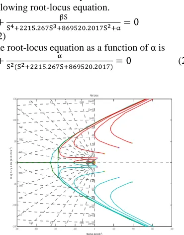
[image:5.612.101.286.240.476.2]Figure 8 Root Contours of the BLDC drive system
Figure 9 Relation between α and Ts
The root-contour plot when β and α as a variable
parameter is shown in the Figure.8. From the root-contour plot it can be seen that the threshold value
of α at which the system will become stable and
unstable is obtained as 0.19×10¹². The root-locus
shown in the right hand side is an unstable one and
the corresponding value of α is 0.4×10¹². Also,
when the parameter α is decreased, the system
becomes more stable. For example, when α =
5×10¹⁰ the system becomes stable for the parameter
β which lies in the range 1.36×10⁸ to 1.72×10⁹.
Also, )*+ (24)
The relationship between α and Ts is depicted in
Figure 9. Ts becomes very small in the millisecond
range when α is greater than 5×10⁹.
6. STEADY-STATE ERRORS AND ERROR CONSTANTS
Steady-state errors constitute an extremely
important aspect of BLDC drive system
performance. The steady-state performance of the drive system can be judged by its steady state error to step, ramp and parabolic inputs. Based on block diagram shown in Figure.3 one can calculate the
steady-state error ωe(s) due to unit step input, ramp
input and parabolic input [8], [9]. Steady- state errors for various inputs are summarized in Table.2.
Table.2 Steady-state errors for various inputs
Type of input Error constants Steady-state error
Unit - step Kp = ∞ 0
Unit - ramp Kv = 0.298 3.35
Unit - parabolic Ka = 0 ∞
From the foregoing analysis, it is seen that the higher the error constants, the smaller the steady-state error. This type-4 system can follow a step-input with zero actuating error at steady state. This drive system can follow the ramp input with a finite error. This analysis also indicates that the BLDC drive system is incapable of following a parabolic input.
7. CONCLUSION
In this paper the relative stability and the transient performance of BLDC drive system are analyzed using Root- Locus method. Also, the movements of the characteristic roots on the s-plane are investigated by varying the system parameter gain. In this paper, the root-contour of the closed-loop BLDC system is plotted to investigate the
effect of variation of parameters α and β. Finally
the steady state error of the system to various standard test signals was outlined in this paper.
From the foregoing analysis it can be concluded that the value of gain k should lie
-400 -300 -200 -100 0 100 200 300 400
-1500 -1000 -500 0 500 1000 1500 0.045 0.1 0.15 0.22 0.3 0.42 0.58 0.85 0.045 0.1 0.15 0.22 0.3 0.42 0.58 0.85 200 400 600 800 1e+003 1.2e+003 1.4e+003 200 400 600 800 1e+003 1.2e+003 1.4e+003 Root Locus
Real Axis (seconds-1)
[image:5.612.90.290.509.663.2]ISSN: 1992-8645 www.jatit.org E-ISSN: 1817-3195
between 0 and 7.561×10¹¹ for the stable operation
of the BLDC drive system. The open-loop poles s3,
s4 and the open-loop zero s5 is too much far away
from the origin. When k increases, they move in left hand side of real axis only. Therefore, these poles and zero has no significant effect on the performance of the drive system. Also, the root loci
cross the imaginary axis at ωn =0.999rad/sec and
the gain value corresponding to the crossing points
is obtained as 7.56×10¹¹. From the root contour
analysis, it can be concluded that the threshold
value of parameter α at which the system will
become stable and unstable is 0.19×10¹². Also, the
BLDC drive system becomes more stable with
reduction in one of the parameter α. The time
constant Ts of the PI controller becomes very small
when α is greater than 5×10⁹.
Also the steady state performance of the system is analyzed by calculating its steady state error for step, ramp and parabolic inputs. The steady state errors for various signals are shown in the table.2. The static error constants are obtained
as Kp=∞, Kv=0.298 and Ka=0. Thus we can
concluded that the higher the static error coefficients, the smaller the steady state error. Also, the BLDC drive system can follow a step input with zero actuating error at stead y state and is incapable of following a parabolic input. This drive system can follow the ramp input with a finite error. This error can be reduced when Kv is increased.
It is concluded that the root –locus method is a powerful and useful approach for the analysis and design of closed-loop BLDC drive system. The root contours are helpful for the study of closed-loop BLDC drive system when other system parameters are to be varied. A quantitative measure of the performance of the BLDC drive system can be achieved with these analyses. These design and analysis of closed loop BLDC drive is helpful to adjust the closed-loop performance of the drive to meet the design specifications
REFERENCES
[1] Anand Sathyan, N.Milivojevic,Y-J Lee and M.Krishnamoorthy, “An FPGA-Based Novel Digital PWM Control Scheme for BLDC Motor Drives” IEEE Trans. on Industrial Electronics”Vol.35, pp 3040-3049 August 2009.
[2] R.C.Becerra and M.Ehsani, “High Speed Torque Control of Brushless PM Motor”
IEEE Trans. on Industrial Electronics, Vol.35, August 1988.
[3] R. Venkitaraman, B.Ramaswami, “Thyristor Converter-Fed Synchronous Motor Drive”, Electric Machines and Electromechanics, 6: 433-449, 1981.
[4] P.Pillay and R.Krishnan, “Modelling,
Simulation, and Analysis of Permanent Magnet Drives, II. The BLDC Motor Drive” IEEE Trans. Indus. Applications, vol.25, No.2,pp 274-279,Mar/Apr. 1989.
[5] M.Ashabani, A.K.Kavani, J.Milimonfared, B.Abdi and Tehron, “Minimization of Commutation Torque Ripple in Brushless DC Motors with Optimized Voltage Control”, IEEE International Symposium on Power Electronics, Electrical Drives, pp 250-255 2008.
[6] Chung-Feng Jeffrey Kuo, Chih- Hui Hsu “Precise Speed Control of a Permanent Magnet Synchronous Motor”, Int. J Adv Manuf Technol. 28: 942-949, May 2005. [7] Ching-Tsai Pan, Emily Fang, “A
Phase-Locked-Loop-Assisted Internal Model Adjustable-Speed Controller for BLDC Motors”,IEEE Trans. On Industrial Electronics, Vol.55, No.9, pp 3415-3425, Sep 2008.
[8] Katsuhiko Ogata, Modern Control Engineering (International Edition) Prentice- Hall of India, New Delhi 1988.
[9] I.J Nagrath and M.Gopal, Control Systems Engineering, New Age International (P) Limited, New Delhi, December 1981.
[10] R.Krishnan,” Electric Motor Drives,
Modelling, Analysis and Control”, PHI Learning Private Limited, New Delhi, 2009. [11] F.Rodigeuz, P.Desai and A.Emadi, “A Novel
Digital Control Technique for Trapezoidal Brushless Dc Motor Drives”, in Proc. Electron, Technol. Conf., Chicago, IL, Nov. 2004.
[12] F.Rodigeuz, and A.Emadi, “A Novel Digital Control Technique for Brushless Dc Motor Drives : Conduction-angle control”, in Proc. IEEE Int. Elect. Mach. Drives Conf.., pp 308-314, May 2005.