Forecasting financial failure using a
Kohonen map: A comparative study to
improve model stability over time
du Jardin, Philippe and Severin, Eric
EDHEC Business School
28 June 2011
1 2 3 4 5 6 7 8 9 10 11 12 13 14 15 16 17 18 19 20 21 22 23 24 25 26 27 28 29 30 31 32 33 34 35 36 37 38 39 40 41 42 43 44 45 46 47 48 49 50 51 52 53 54 55 56 57 58 59 60 61
Forecasting financial failure using a Kohonen map: A comparative study to
improve model stability over time
Philippe du Jardina,1,∗, Eric S´everinb,2
a
Edhec Bussiness School, 393 Promenade des Anglais, BP 3116, 06202 Nice Cedex 3, France
b
Universit´e de Lille 1, 104 Avenue du Peuple Belge, 59000 Lille, France
Abstract
This study attempts to show how a Kohonen map can be used to improve the temporal stability of the accuracy of a financial failure model. Most models lose a significant part of their ability to generalize when data used for estimation and prediction purposes are collected over different time periods. As their lifespan is fairly short, it becomes a real problem if a model is still in use when re-estimation appears to be necessary. To overcome this drawback, we introduce a new way of using a Kohonen map as a prediction model. The results of our experiments show that the generalization error achieved with a map remains more stable over time than that achieved with conventional methods used to design failure models (discriminant analysis, logistic regression, Cox’s method, and neural networks). They also show that type-I error, the economically costliest error, is the greatest beneficiary of this gain in stability.
Keywords: decision support systems, finance, bankruptcy prediction, self-organizing map
1. Introduction
Models that have long been used by banks and rating agencies to forecast firm failure, have many drawbacks that have given rise to an extensive body of literature (Balcaen and Ooghe, 2006). Nearly all of the drawbacks (whether related to modelling techniques, sampling and variable selection procedures, control parameters, model design or validation processes) that could have an effect on their robustness have been analysed. But one of these drawbacks, having to do with data stationarity, has not been overcome. A forecasting model relies on the assumption that the relationship between the dependent variable (i.e. failure probability) and all independent variables
∗Corresponding author
Email addresses: [email protected](Philippe du Jardin),[email protected] (Eric S´everin)
1
Tel.: +33 (0)4 93 18 99 66 - Fax: +33 (0)4 93 83 08 10
2
4 5 6 7 8 9 10 11 12 13 14 15 16 17 18 19 20 21 22 23 24 25 26 27 28 29 30 31 32 33 34 35 36 37 38 39 40 41 42 43 44 45 46 47 48 49 50 51 52 53 54 55 56 57 58 59 60 61
is stable over time (Zavgren, 1983). Yet there is evidence that this stability is highly questionable (Charitou et al., 2004) and that the true forecasts of a model may be weak if this assumption is not fulfilled (Mensah, 1984). Indeed, models are sensitive to some parameters that describe macro-economic environments, and any change may influence their accuracy (Mensah, 1984; Platt et al., 1994). In practice, then, models need to be re-estimated frequently to counterbalance the effects of such phenomena (Grice and Ingram, 2001). However, nobody knows what their life span is, how often they need to be re-estimated. This uncertainty has a cost, the cost of the error made when a model unexpectedly enters its instability zone, and especially the cost of type-I errors, that is, the cost of predicting that a firm will survive when in fact it will go bankrupt. In such circumstances, the potential cost for an investor or a creditor who decides, for example, to lend money based on a bankruptcy risk probability involves a net loss in capital that will not be reimbursed, whereas type-II errors involve only the loss of a commercial bargain. For these reasons, we study a means to improve model stability over time.
Two main parameters lie at the root of model instability when there is a change in the economic environment between the period during which a model is estimated and that during which it is used for prediction. Firstly, the boundary that makes it possible to discriminate between healthy and unsound companies moves slightly (Pompe and Bilderbeek, 2005). Secondly, the distribution of explanatory variables changes (Pinches et al., 1973); variable mean and standard deviation are no longer identical and this phenomenon influences model accuracy. In this study, we focus on the latter issue so as to mitigate the effect of sampling variations. Instead of using financial indicators as explanatory variables, we proposed using them in a different way: these financial variables were used to design a set of regions at risk and to compute the ways companies moved within these regions over time. These moves were then quantified to represent standard behaviours, called “trajectories”, and these trajectories were used to make forecasts. We thus developed a typology of behaviours, some leading to bankruptcy, others not, and we studied both their forecasting ability and their ability to provide estimates less sensitive to macro-economic changes than those of traditional models. Regions at risk and trajectories were designed using Kohonen maps, and the prediction ability of trajectories was compared to that of models designed using discriminant analysis, logistic regression, Cox’s method and a neural network3. We made these comparisons with data collected over different time periods, experiencing various economic conditions; models were estimated with data collected
3
4 5 6 7 8 9 10 11 12 13 14 15 16 17 18 19 20 21 22 23 24 25 26 27 28 29 30 31 32 33 34 35 36 37 38 39 40 41 42 43 44 45 46 47 48 49 50 51 52 53 54 55 56 57 58 59 60 61
over periods of either economic growth or downturn, and their prediction ability was assessed with data collected over similar or dissimilar periods.
The remainder of this paper is organised as follows. In section 2, we present a literature review that explains our research question. In section 3, we describe the samples and methods used in our experiments. In section 4, we present and discuss our results and in section 5, we conclude and suggest further research.
2. Literature review
Most financial failure prediction models rely on regression or classification techniques and were designed with single-period data. A model makes it possible to forecast the fate of a company at timet depending on data measured at timet−1. It is therefore assumed that, between the point in time when the regression or classification function is estimated and that when the function is to be used for a prediction purpose, the relationship between a probability of failure and variables used to compute it (financial ratios, for the most part) is stable (Mensah, 1984). It is also assumed that the extent to which variables are correlated does not change (Zavgren, 1983). However, it has been shown that these assumptions do not hold (Altman and Eisenbeis, 1978). Indeed, both the relationship between the dependent and independent variables and the distribution of explana-tory variables are likely to be influenced by macro-economic phenomena. Therefore, any change in environmental conditions may greatly reduce model accuracy. It has been demonstrated that variations in economic cycles (alternating periods of economic growth and downturn or recession) and, to a lesser extent, changes that firms may face in terms of interest rates, credit policy, tax rates, competitive structures, technological cycles and institutional environment, have an influence on financial ratio distributions and on the boundary between failed and non-failed companies. This influence may result in models having poor prediction abilities (Mensah, 1984; Platt et al., 1994; Grice and Dugan, 2003). Of course, other parameters may play a role, especially when models are used with data that are outside their scope of validity. This is the case when a model is designed for a given firm’s size (or for a particular sector or country) and is used with companies that do not meet these criteria. But the latter parameters are easily monitored and controlled, unlike the former.
4 5 6 7 8 9 10 11 12 13 14 15 16 17 18 19 20 21 22 23 24 25 26 27 28 29 30 31 32 33 34 35 36 37 38 39 40 41 42 43 44 45 46 47 48 49 50 51 52 53 54 55 56 57 58 59 60 61
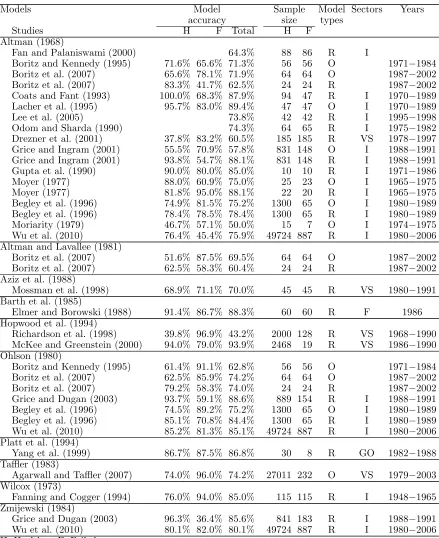
literature. This table includes Altman’s (1968), Wilcox’s (1973), Ohlson’s (1980), Taffler’s (1983) and Zmijewski’s (1984) models, which are among the most popular. It also shows the correct classification rates of healthy and failed companies that are achieved with each model, including the sample size used to test model accuracy, companies’ sectors of operations, and the time period during which data were collected.
Table 2 shows the different studies that assessed the prediction performance of all these models under the same conditions as those used when they were designed (identical modelling technique, identical sector), except the time period during which data were collected. And models were eval-uated either in their original form or in a re-estimated form. All but two studies achieved correct classification rates far lower than those reported by their initial authors. Altman’s (1968) model, which originally had an accuracy rate of 95.5%, ultimately had an accuracy rate ranging from 85% to 89.4% with five studies, and less than 80% with thirteen others. The results achieved with other models are similar. However, when original model coefficients are re-estimated to cope with the characteristics of the period during which they were used once again, models achieved rather better results. Four of the five studies that use Altman’s (1968) model, and that achieve the best results, managed to do so with a re-estimated function. The same conclusion can be drawn from the results achieved with Ohlson’s (1980) model. As far as the others are concerned, except Barth et al.’s (1985) model, used by Elmer and Borowski (1988), and Hopwood et al.’s (1994) model, used by McKee and Greenstein (2000), they all lead to the conclusion that the difference between the performance of a model, as originally reported, and the performance achieved, with a new sample, is fairly clear. These tables show clearly why failure models must be re-estimated frequently. They also show the limits of traditional validation procedures, where models are tested with samples col-lected within the same timeframe as that used to estimate them. However, no one knows how often such a re-estimation is to be done, even if it is clear that the more complex a classifier, the more often it must be re-estimated (Finlay, 2011). This fact is not without consequences for banking and financial institutions when some of their decisions are based on the evaluation of a risk calculated with this kind of model.
4 5 6 7 8 9 10 11 12 13 14 15 16 17 18 19 20 21 22 23 24 25 26 27 28 29 30 31 32 33 34 35 36 37 38 39 40 41 42 43 44 45 46 47 48 49 50 51 52 53 54 55 56 57 58 59 60 61
applicable onlya posteriori when one knows what the nature of the macro-economic changes was, and thus how to mitigate their effects. But, a priori, no one knows what should be done. Other authors demonstrated that one could take advantage of sampling variations caused by changes in the economic environment, and that one might improve model accuracy in the short term by using measures representing variation of ratios over time (standard deviation, coefficient of variation), but they did not study the stability of model accuracy in the long term (Dambolena and Khoury, 1980; Betts and Belhoul, 1987).
The latter approach implicitly acknowledges that the temporal stability of a model might be im-proved by using data collected over several consecutive years. This idea is close to the fact that history is a critical explanatory “variable” of business survival. Indeed, one knows that bankruptcy, in most cases, is the result of a long process (Laitinen, 1991), and that a firm’s history strongly influences its ability to withstand failure. Thus, some companies can delay the onset of bankruptcy for many years, even though their financial profile shows that they should fail rapidly, whereas oth-ers manage to recover even though nothing suggests that an improvement may happen (Hambrick and D’Aveni, 1988). A firm’s financial health measured at timetcannot be reduced to its situation measured at time t−1 alone, although this is the underlying assumption of most failure models. However, this idea has been little explored so as to improve model accuracy (Balcaen and Ooghe, 2006), and even less to increase their stability over time
4 5 6 7 8 9 10 11 12 13 14 15 16 17 18 19 20 21 22 23 24 25 26 27 28 29 30 31 32 33 34 35 36 37 38 39 40 41 42 43 44 45 46 47 48 49 50 51 52 53 54 55 56 57 58 59 60 61
failure and the performance achieved with trajectories was compared to that achieved using tra-ditional failure models that were designed with discriminant analysis, logistic regression, survival analysis (Cox’s method) and a neural network. As we looked at the influence of economic cycles on the stability of results, which appear to be the main factor of data non-stationarity, models were estimated and tested using data collected from different time periods (growth and downturn).
3. Samples and methods
Data were selected from a French database (Diane), which provides financial data on more than one million French firms. We only chose companies required by law to file their annual reports with the French commercial courts. We also chose companies in the same activity (retail) and of the same size (assets less than e750,000), to control for size and sector effects. We only selected
income statement and balance sheet data, which have been the main sources of information for failure models since Altman (1968). This set of data was used to calculate ratios, and these ratios were subsequently used to design models. As we needed sufficient data to compute trajectories, we selected companies in operation for at least six years, keeping the same time frame as Laitinen (1991).
3.1. Covered periods
To collect data from different economic periods, we analysed changes in the French economic situation between 1991 and 2009. Over these 19 years, France experienced two recessionary periods and one downturn period4. The first recession occurred between March 1992 and June 1993, the downturn5 occurred between March and December 2001, and the second recession began in March 2008. Figure 1 shows the changes in both gross domestic product (GDP) and business failure growth rates between 1991 and 2009, and clearly illustrates how downturns were preceded and followed by periods of growth, some more pronounced than others. We noticed a period of recovery and growth between 1993 and 2000, after the 1992 recession, despite a slight fall in GDP in 1996. In addition, the downturn which occurred in 2001 had an influence on the economy until late 2002, and growth slowly resumed in 2003 and continued to increase until early 2008.
4
For economists, a recession occurs if GDP (gross domestic product) growth is negative for two or more consecutive quarters.
5
4 5 6 7 8 9 10 11 12 13 14 15 16 17 18 19 20 21 22 23 24 25 26 27 28 29 30 31 32 33 34 35 36 37 38 39 40 41 42 43 44 45 46 47 48 49 50 51 52 53 54 55 56 57 58 59 60 61
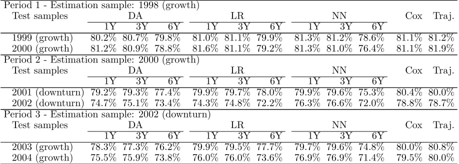
The different time periods during which we collected data were chosen based on Figure 1. We chose three periods; hence we designed three sets of models. The first was calculated with data collected from 1998 and was tested with data from 1999 and 2000 (estimation and test over a period of growth). The second set was calculated with data collected from 2000, and tested with data from 2001 and 2002 (estimation over a period of growth, and test over a period of downturn). Finally, the third set was designed using data collected from 2002, then tested with data from 2003 and 2004 (estimation over a period of downturn and test over a period of growth).
We wished to analyse model performance using data collected over a downturn period, either for estimation and test purposes. This would have required the downturn period to last at least three years: one year to collect data for estimation tasks, and the following two years to collect data for prediction tasks. Unfortunately, no recessionary or downturn periods that occurred in France between 1990 and 2011 have lasted this length of time. The recessions that occurred between 1992 and 1993 and between 2008 and 2009 are both immediately followed by a period of growth. And the situation is the same after the downturn that occurred between 2001 and 2002, with 2003 also being a period of growth.
3.2. Sample selection
We selected seven samples. Table 3 shows the years for which we collected data, the number of companies per sample and how samples were used for estimation or prediction tasks or both. For each sample collected at timet, company status (healthy vs. failed) was assessed at timet+ 1, with an average lag of 12 to 18 months. Balance sheets and income statements were selected from six consecutive years (t to t−5) and firms were chosen at random from among those in the database when they complied with the criteria described above.
3.3. Variable selection
Choosing a subset of variables from an initial set is essential to the parsimony of a model, but also essential for its accuracy and generalization ability. This task is difficult because the evaluation criterion used to select variables is often non-monotone. Indeed, the best subset of p
4 5 6 7 8 9 10 11 12 13 14 15 16 17 18 19 20 21 22 23 24 25 26 27 28 29 30 31 32 33 34 35 36 37 38 39 40 41 42 43 44 45 46 47 48 49 50 51 52 53 54 55 56 57 58 59 60 61
explores a subspace of all possible combinations and generates a set of candidate solutions; an evaluation criterion to evaluate the subset under examination and select the best one(s); a stopping criterion to decide when to stop the search method.
When the evaluation criterion is monotone, “complete” methods may find an optimal solution without evaluating all possible combinations, like Branch and Bound (Narendra and Fukunaga, 1977). Several variants derived from Branch and Bound can deal with situations where the criterion is non-monotone. With some of them, such as Approximate Monotonic Branch and Bound, the optimality of the solution is no longer guaranteed. However, with some others (Duarte Silva, 2001; Brusco and Steinley, 2011), the optimality can be reached but the size of the set of variables must be limited. These latter methods offer a valuable alternative to sequential methods, including stepwise methods, which usually only find local minima, but they work well only with a moderate number of variables (between 30 and 50) so that the computation times are not prohibitive.
Heuristic or “sequential” methods are used to relax the monotonic assumption that Branch and Bound imposes on the evaluation criterion and represent an alternative to complete methods, which are able to find a global minimum, when the number of variable is large. The simplest methods start with an empty set of variables, then add them one at a time (forward search); others start with all variables, then remove them, also one at a time (backward search). These methods produce results quickly, but they lead to non-optimal solutions because they search only a small part of the space. To increase the size of the search space, some methods such as Plus l – Take Away r alternate forward and backward steps (stepwise methods). Others called floating methods, derived from Plus l – Take Away r, also alternate forward and backward steps, but using a constraint on the evaluation criterion. Their advantage lies in dynamically determining the number of variables that are to be added or removed, as opposed to others where this number is fixed a priori (Jain and Zongker, 1997).
Finally, “random” methods reduce the risk of a method getting trapped in a local minimum. They start by choosing at random a set of variables, and then search using either a sequential strategy (Simulated Annealing) or a random one (genetic algorithms).
4 5 6 7 8 9 10 11 12 13 14 15 16 17 18 19 20 21 22 23 24 25 26 27 28 29 30 31 32 33 34 35 36 37 38 39 40 41 42 43 44 45 46 47 48 49 50 51 52 53 54 55 56 57 58 59 60 61
Wilks’ Lambda), information measures (entropy), dependence measures (mutual information) or consistency measures. When used in conjunction with some algorithms, these criteria do not always lead to optimal results, or they are difficult to use. Therefore, one uses the induction algorithm (Kohavi and John, 1997) for evaluation: each set of variables selected at any given time is then evaluated based on the generalization error of the model designed with these variables.
Without a suitable stopping criterion, a selection process could run until all possible combinations are evaluated. Many criteria may be used to interrupt a search. Most of the time these criteria take the form of a maximum number of iterations, a predefined number of variables, the absence of improvement after addition or removal of variables, or the achievement of optimal predictive ability. These criteria depend on computation heuristics and sometimes on statistical tests. When it comes to choosing a variable selection method, one has to therefore choose a combination of three of the aforementioned techniques and criteria – a choice that is not necessarily straightforward. Indeed, depending on the selection method being considered, some techniques or criteria that have just been presented cannot be used, either because they are difficult to implement and cause intractable computational problems, or because they are ill-suited to the modelling technique. This is, for example, the case of evaluation criteria that rely on the hypothesis that input-output variable dependence is linear or that input variable redundancy is well measured by the linear correlation of these variables, and that are clearly not suited to neural networks (Leray and Gallinari, 1998). And even if the selection technique fits the modelling method, the question of the final choice and that of the role of the user in this choice always arises. This is the reason why some authors suggest that several criteria should be used simultaneously to select variables and that a certain degree of subjectivity might be involved in the selection process (Duarte Silva, 2001).
As a consequence, we used several selection methods and only variables that were most often selected were finally chosen to design our models. This approach corresponds to the idea proposed by (Murray, 1977) who thought that a good measure of the value of a variable for future classification would be the number of times it was selected by different techniques. The selection process was therefore organized as follows.
4 5 6 7 8 9 10 11 12 13 14 15 16 17 18 19 20 21 22 23 24 25 26 27 28 29 30 31 32 33 34 35 36 37 38 39 40 41 42 43 44 45 46 47 48 49 50 51 52 53 54 55 56 57 58 59 60 61
subset with data from 1998 (period of growth), a second subset with data from 2000 (period of growth) and a third with data from 2002 (period of downturn). For each period, we used the following procedure to select variables.
We chose six variable selection techniques commonly used with the modelling methods we chose for our experiments. We selected three techniques that are commonly used with discriminant analysis, logistic regression and Cox’s method, and three others that are well suited for the neural network (multilayer Perceptron). We did not choose any method dedicated to Kohonen maps. Indeed, the way we used these maps is very different from the way they are traditionally used and therefore, there was no guarantee that a variable selection method tailored to Kohonen maps would have been, within the framework of our study, more useful than another.
4 5 6 7 8 9 10 11 12 13 14 15 16 17 18 19 20 21 22 23 24 25 26 27 28 29 30 31 32 33 34 35 36 37 38 39 40 41 42 43 44 45 46 47 48 49 50 51 52 53 54 55 56 57 58 59 60 61
each set of variables, we tested several combinations of parameters: learning steps (from 0.05 to 0.5, with a 0.05 step) and the number of hidden nodes (from 2 to 15). We used only one hidden layer. All these figures were derived from those traditionally used with an MLP in the literature. For each combination of parameters, the error was estimated using a 10-cross-validation technique and the architecture that led to the lowest error was chosen. All networks used in this study were made up of one hidden layer, one output node and an activation function in the form of a hyperbolic tangent. We used the Levenberg-Marquardt algorithm, as an optimization technique during the learning process.
When all selections were done with each method, variables that were selected at least twice were chosen to design our models, but highly correlated variables were removed because correlation leads to model instability (Mensah, 1984). When the correlation between two variables was greater than 0.7, one of them was removed. We chose 0.7 as Atiya (2001) and Leshno and Spector (1996) did in the same context as that of this study. When deciding on which variables to remove, we used the following procedure. When one of the two variables was likely to give too much weight to a given financial dimension among those that were represented in a set of variables, it was discarded. The financial dimensions that are most often captured by variables used to design bankruptcy models are liquidity, solvency, profitability and financial structure, as suggested by many authors since Gupta (1969). We then managed to balance the weight of each main dimension captured by each set of variables. But when neither of the two variables was likely to overweight any given dimension, the variable that appeared to be the less “relevant” in the financial literature, given the issue we studied, was removed. The fact that a variable belonged to a certain financial dimension was assessed using the financial literature and confirmed using a principal component factor analysis.
3.4. Modelling methods
Several modelling methods were used to design prediction models: a Kohonen map, to calculate trajectories, and three traditional methods such as discriminant analysis, logistic regression and a neural network.
4 5 6 7 8 9 10 11 12 13 14 15 16 17 18 19 20 21 22 23 24 25 26 27 28 29 30 31 32 33 34 35 36 37 38 39 40 41 42 43 44 45 46 47 48 49 50 51 52 53 54 55 56 57 58 59 60 61
this difference between data used with each method (single period data vs. time-series data), we designed several multi-period models. We first used a survival analysis (Cox’s method) which is specially designed to deal with time-series data. This method was used with data measured over six years. Secondly, we added models designed with discriminant analysis, logistic regression and the neural network that used data collected over different time periods. With these models, each explanatory variable was measured at different points in time. For example, a model that was designed with five financial ratios and that used data collected over six years is made up of thirty explanatory variables. We used two time periods (three and six years) to control for the influence of the number of variables on model accuracy, that is to say the influence of the number of parameters to be estimated. Indeed, in general, the more parameters to be estimated on a given data set, the greater the generalization ability of a model is difficult to achieve.
3.4.1. Discriminant analysis
Discriminant analysis is a classification method with the aim of classifying objects in two or several groups using of a set of variables. To design the classification rule, the method attempts to derive a linear combination of independent variables that will best discriminate between previously defined groups, which in our case are sound and unsound firms. This is achieved using a procedure of maximizing the between-group variance relative to the within-group variance. Discriminant analysis then computes a scorez according to:
z=
n
X
i=1
(xiwi+c) (1)
wherewi represents the discriminant weights,xi indicates the independent variables (e.g., financial
ratios) andcis a constant. Each firm is assigned a single discriminant score which is then compared to a cut-off value which determines the group the company belongs to.
4 5 6 7 8 9 10 11 12 13 14 15 16 17 18 19 20 21 22 23 24 25 26 27 28 29 30 31 32 33 34 35 36 37 38 39 40 41 42 43 44 45 46 47 48 49 50 51 52 53 54 55 56 57 58 59 60 61
3.4.2. Logistic regression
Logistic regression is often used in conjunction with or instead of discriminant analysis to relax the conditions for optimality that the latter method imposes on the data. This is particularly the case when variables used to design models, such as financial ratios, exhibit characteristics that depart severely from these conditions.
A logistic regression function computes a probability score z for each observation (firm) to be classified, where:
z= 1
1 +e−Pni=1(xiwi+c)
(2)
where xi represents the independent variables and c is a constant. The coefficients wi of the
function are calculated using maximum likelihood estimation. As with a discriminant function, an observation will be classified in one of two groups depending on its score.
3.4.3. Neural network
Neural networks, like discriminant analysis or logistic regression, are commonly-used classifi-cation methods in the field of bankruptcy prediction. Unlike discriminant analysis and logistic regression, neural networks do not represent the relationship between the independent variables and the dependent variable with an equation. This relationship is expressed as a matrix containing values (also called weights) that represent the strength of connections between neurons. In this study, a multilayer Perceptron (MLP) was used to perform the classification task. From a general point of view, a MLP used for classification tasks with two groups is made up of three layers: an input layer withnneurons, one per explanatory variable; one hidden layer withmneurons; and an output layer with one neuron. The layers are linked together, and the relationships between neurons are represented by weights: the weights w1ij represent the relationships between the neurons of the input layer (xi) and the neurons of the hidden layer. The weights w2j represent the relationships
between the neurons of the hidden layer (hj) and the output neuron.
If one considers a classification task of observations into two groups to be achieved by such network, the vector x represents the explanatory variables, and the output neuron represents the result of the classification: class 1 or class 2. The values go through the network as a result of the activation function of each neuron. The activation function transforms input into output. The input value of a hidden neuron (hj) is the weighted sum of the input neurons Pni=1(xiwij1) and its output is
f(Pn
i=1xiw1ij). The output of the output neuron isf(
Pm
j=1hjw2j). The transformation of the input
4 5 6 7 8 9 10 11 12 13 14 15 16 17 18 19 20 21 22 23 24 25 26 27 28 29 30 31 32 33 34 35 36 37 38 39 40 41 42 43 44 45 46 47 48 49 50 51 52 53 54 55 56 57 58 59 60 61
transformation allows the network to take into account the non-linearity that may exist between its input and its output. The weights of the network are estimated through a learning process. During this process, network weights are tuned to values that allow the network to achieve a good classification rate with data used during the learning phase, but also good prediction ability when using data that were not used during this phase. Once the learning process is done, the network can be used for forecasting tasks.
An MLP does not require distributional assumptions of the independent variables and is able to model all types of non-linear functions between the input and the output of a model. This univer-sal approximation capability, assessed Hornik et al. (1990), and the ability to build parsimonious classification rules make them powerful models.
3.4.4. Cox’s method
Cox’s method is one of the techniques known as survival analysis which allows the time that will elapse before a particular event occurs, such as bankruptcy, to be taken into account. This method is completely different from the previous ones. With discriminant analysis, logistic regression or neural networks, bankruptcy prediction is achieved using a classification rule. With a Cox’s model, bankruptcy prediction is done using a timeline over which a firm is characterized by a specific lifetime. Lifetime distributions in a given population can be represented by two functions: a survival function and a hazard function. The survival functions(t) represents the probability that a firm will survive past a given time t, and the hazard function h(t) represents the instantaneous rate of failure at a given time t. There are different ways of assessing the survival and the hazard functions that depend on the assumptions about the relationships between these functions and a set of explanatory variables. With Cox’s method, this relationship can be represented as:
h(t) =h0(t)e
Pn
i=1xiwi (3)
where h0(t) corresponds to the baseline hazards and describes how the hazard function changes
over time andePni=1xiwi corresponds to the way the hazard function relates to explanatory variables
xi. The regression coefficients wi are calculated with a method similar to the maximum likelihood
method.
The survival function s(t) of a given company can be defined as:
4 5 6 7 8 9 10 11 12 13 14 15 16 17 18 19 20 21 22 23 24 25 26 27 28 29 30 31 32 33 34 35 36 37 38 39 40 41 42 43 44 45 46 47 48 49 50 51 52 53 54 55 56 57 58 59 60 61
As with a discriminant or a logistic function, a firm will be classified in one of two groups depending on its survival function.
3.4.5. Kohonen maps
Kohonen maps were originally designed to deal with clustering issues. A map consists of a set of neurons organised on a square grid most of the time. Each neuron is represented by an n-dimensional weight vector w= (w1, . . . , wn), wheren is the dimension of the input vectors (i.e.
number of variables used to represent observations). The weights of a map are calculated through a learning process during which the neurons learn the underlying patterns within the data. During this process all data vectors are compared to all weight vectors through a distance measure. For each input vector, once the nearest neuron is found, its weights are adjusted so as to decrease the distance between the input vector and this neuron. The weights of all neurons located in its neighbourhood are then also adjusted, but the magnitude of the variation is proportional to the distance between them on the map. Throughout the learning phase, the neighbourhood radius gradually shrinks, depending on a function to be defineda priori. This procedure is repeated until a stopping criterion is reached.
When the learning process is done, the resulting map is a non-linear projection of an n-dimension input space onto a two-dimensional space, which preserves the structure and topology of input data relatively well (Cottrell and Rousset, 1997): two companies that are close to each other in the input space will be close on the map. As the classes are known (failures vs. survivors), each neuron can be labelled with the label of the class for which it appears as a prototype. To do so, all input vectors are once again compared to all neurons. The percentage of companies in each class that are the closest to each neuron is then computed. Finally, the neurons are labelled with the label of the class whose percentage is the highest. The algorithm used during the learning phase of the map can be described as follows:
• Step 1: set the size of the map, using l lines and c columns, then randomly initialize the weights;
• Step 2: set the input neuron valuesx= (x1, . . . , xn) using data from one company;
• Step 3: compute the distance between vector (x1, . . . , xn) and the weight vector (xk1, . . . , wkn)
of each neuronwk and select neuronwc with the minimum distance:
4 5 6 7 8 9 10 11 12 13 14 15 16 17 18 19 20 21 22 23 24 25 26 27 28 29 30 31 32 33 34 35 36 37 38 39 40 41 42 43 44 45 46 47 48 49 50 51 52 53 54 55 56 57 58 59 60 61
• Step 4: update weights within the neighbourhood ofwc:
wk(t+ 1) =wk(t) +α(t)hck(t)[x(t)−wk(t)]
wheretis time, α(t) the learning step,hck(t) the neighbourhood function, andx(t) the input
vector. The neighbourhood function is traditionally a decreasing function of both time and the distance between any neuron wk on the map and neuron wc that is the closest to the
input vector at timet.
• Step 5: repeat step 2 to step 5 until treaches its final value.
3.4.6. Kohonen map and trajectory design
A trajectory represents the variation of company’s financial health over time. It also represents the way a firm moves in at-risk regions, over a number of consecutive years. A trajectory is then a sequence of positions within a space at risk, over a given period. We used a Kohonen map to design the space at risk, and a few others to design trajectories.
A map made up of 100 neurons was used to design the space at risk – 10 per row and 10 per column6. Three different spaces were then designed: one with data from 1998; one with data from
2000; and a last one with data from 2002. We used Sammon’s mapping method (Sammon, 1969) to make sure that the input space was well approximated with a two-dimensional map and that no significant folding or stretching was visible on the map
Once the design of each map was completed,7, we looked for neurons that can be considered
pro-totypes of healthy and failed firms. To do so, we compared data used to design the maps and all neurons. We then calculated the percentage of sound and unsound firms that were closest to each neuron. Finally, neurons were labelled with the label of the class (healthy or failed) whose percentage was higher. When neurons are labelled, the map can be used to visualize the location of companies belonging to each class. It gives a complete picture of the proximity between failed and non-failed firms on the map, and makes it possible to represent a “failure” and a “non-failure space” and the boundaries between them.
Once the map was designed, company trajectories were computed: a trajectory is a path along which a company moves on the map from one neuron to another (i.e. from one region at risk to another) over a six-year period. These at-risk regions can be considered the hierarchies of finan-cial profiles that best summarize all company finanfinan-cial situations. As we have collected data over
6
This figure is somewhat arbitrary but it corresponds to usual empirical practices (Cottrell and Rousset, 1997).
7
4 5 6 7 8 9 10 11 12 13 14 15 16 17 18 19 20 21 22 23 24 25 26 27 28 29 30 31 32 33 34 35 36 37 38 39 40 41 42 43 44 45 46 47 48 49 50 51 52 53 54 55 56 57 58 59 60 61
six-year periods, each company can be represented using six vectors, one for each year. To locate the position of a company on the map, we computed the distance between all neurons and the six vectors. The neurons that are the closest to each vector then represent the different positions of a company on the map over time. Each sequence of six positions can be considered a trajectory. However, as a map is made up of 100 neurons, it becomes impossible to analyse and visualize all possible trajectories. To reduce the number of combinations, we attempted to group neurons into a few super-classes. Each class of neurons was analysed separately to look for groups only repre-senting healthy companies, and other groups only reprerepre-senting unhealthy companies. Neurons were then grouped into a small number of groups called super-classes8 using a hierarchical ascending classification9.
We then ranked the super-classes by the financial health of the companies they represented, ranging from companies in very good shape (super-class 1) to those in very bad shape (super-class n, n>1). Financial ratios were used to establish the hierarchy. Once established, we computed the different trajectories in keeping with the initial position of each company on the map over the first year of each period studied (that is, the positions in 1993, 1995 and 1997). We first calculated company trajectories whose initial positions in 1993, 1995 and 1997 were super-class 1, then company tra-jectories whose initial positions were super-class 2, etc. There are as many sets of tratra-jectories as super-classes on the map.
Figure 2 depicts three individual trajectories on the map designed with data from 2002. This par-ticular map is made up of 6 super-classes. Super-classes 1, 2, 3 and 4 (healthy zone on the map) represent neurons which encode healthy companies, and super-classes 5 and 6 (bankruptcy zone) represent neurons which encode failed companies. On this map, each set of lines, depicted with a different colour, shows the behaviour of a company. The steps are numbered and each one encodes a position on the map within a year – 1 is the position in 1997, 2 in 1998, 3 in 1999, 4 in 2000, 5 in 2001 and 6 in 2002.
The first trajectory (black lines) exhibits the behaviour of a company (firm 1) that stayed healthy for six years and whose initial (1997) and final (2002) positions on the map was super-class 1. The
8
We analysed a few partitions made up of six to eleven super-classes, and we finally chose the best partition in terms of homogeneity. The homogeneity was assessed using the three best homogeneity indexes mentioned in the research carried out by Milligan (1981).
9
4 5 6 7 8 9 10 11 12 13 14 15 16 17 18 19 20 21 22 23 24 25 26 27 28 29 30 31 32 33 34 35 36 37 38 39 40 41 42 43 44 45 46 47 48 49 50 51 52 53 54 55 56 57 58 59 60 61
second one (gray lines) shows how a company (firm 2) moved slowly along a path to failure from an initial position in super-class 1 to a final position in class 6. In 1997, its situation was fairly good, but as time went by, its financial ratios progressively deteriorated and, finally, it went bankrupt in 2003. The third trajectory (white lines) is rather erratic. This firm (firm 3) was in bad shape in 1997 (initial position in class 5), and managed to recover two years later (position in class 1), but this remission was short. From 2000 to 2001 its situation worsened (position in class 5), only to get better in 2002 (position in class 1).
For each period, when all individual trajectories (one per company) were calculated, we then grouped these trajectories into prototype trajectories – one per super-class. For each super-class, we used a single-layer, six-neuron Kohonen map to compute the prototype trajectories. Six neurons were enough to correctly quantify all data, because, with more than six, some trajectories became indistinguishable from others, and with fewer, some no longer existed. With each learning sample (i.e. data from 1993 to 1998, 1995 to 2000 and 1997 to 2002), all prototype trajectories were la-belled with the label of a class (sound or unsound) depending on a cut-off value described in the next paragraph below. Finally, we grouped all six-neuron maps into a final set (one per period), and we used it to complete the forecasts.
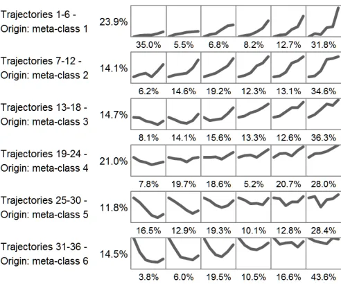
Figure 3 shows the distribution of prototype trajectories designed with the map depicted on Figure 2 over the period from 1997 to 2002. The six lines on Figure 3 display trajectories whose origin is super-class 1, 2. . . , 6 respectively on the map presented on Figure 2. On each graph, the scale of the X-axis corresponds to the six years, and the scale of the Y-axis corresponds to the six super-classes. The percentages shown in the columns are the proportion of companies belonging to each set of trajectories; the percentages shown below each graph represent the same proportion, but within each trajectory.
The first line displays the behaviour of companies belonging to super-class 1, that is, firms with the best financial health. The first four trajectories show that most of these firms never shifted to the “bankruptcy space”, unlike the last two trajectories, which show that some of them ultimately went bankrupt.
4 5 6 7 8 9 10 11 12 13 14 15 16 17 18 19 20 21 22 23 24 25 26 27 28 29 30 31 32 33 34 35 36 37 38 39 40 41 42 43 44 45 46 47 48 49 50 51 52 53 54 55 56 57 58 59 60 61
3.4.7. Cut-off value determination
The cut-off value used to discriminate between sound and unsound firms was calculated with two different methods. A set of forecasts were then made with each method.
Firstly, the cut-off value was estimated so as to maximize the overall rate of correct classifications. This is the most commonly used method in the bankruptcy literature. However, as previously mentioned, since the cost of misclassification between two models that exhibit equal performance is not symmetric, the best option is certainly the model that is able to minimize the type-I error (bankrupt firms predicted as healthy). This is the reason why many authors recommend to taking this cost into account while assessing the optimal cut-off value, and explicitly using it during the computation of a classification function. A second way of assessing the cut-off value was then used to take the observed expected cost of misclassification – also called resubstitution risk – into account (Frydman et al., 1985). Thus, the following objective function was minimized to estimate the cut-off value:
Expected cost =c1p1
e1
N1
+c2p2
e2
N2
(5)
where c1 and c2 are the respective costs of type-I and type-II errors; p1 and p2 are the respective
prior probabilities of bankruptcy and non-bankruptcy; e1 and e2 are the respective type-I (failed
firm predicted as healthy) and type-II (healthy firm predicted as failed) errors; andN1 and N2 are
the respective numbers of failed and healthy firms in the sample.
The main difficulty lies in specifying the values to be used withc1 and c2. Indeed, as suggested by
Pacey and Pham (1990),c1andc2 differ from firm to firm, but also from the situation of the user of
the model and therefore on its own cost-of-error function. We then used the misclassification costs used by Frydman et al. (1985), the aim of whose study was also to compare different bankruptcy prediction models, where the cost of misclassification of healthy firms (i.e., c2) is kept to 1, while
the costs of misclassification of unsound firms (i.e., c1) are respectively set to 1, 10, 20, 30, 40,
50, 60 and 70. As far as the prior probability of bankruptcy is concerned, we used the average probability of French firms belonging to the retail sector over the period studied – that is, 2%. This parameter was also used by Frydman et al. (1985) and by Tam and Kiang (1992).
4 5 6 7 8 9 10 11 12 13 14 15 16 17 18 19 20 21 22 23 24 25 26 27 28 29 30 31 32 33 34 35 36 37 38 39 40 41 42 43 44 45 46 47 48 49 50 51 52 53 54 55 56 57 58 59 60 61
was changed so as to take into account the prior probabilities and the costs of misclassification (Tam and Kiang, 1992). Finally, with the Kohonen map, the cost function was used to label the trajectories that were used to make forecasts, in the same way as terminal nodes of a classification tree are labelled when using such a function (Frydman et al., 1985). Trajectories were labelled with the label of the class (healthy vs. failed) that minimized the observed cost of misclassification. Consider a trajectory t that has to classify ni(t) objects from group i, and let Ni be the size of
group iin the sample, with i= 1,2. The risk of labeling trajectory t with the label of group 1 is defined as:
r1(t) =c2p(2, t) =c2p2p(t|2) =c2p2
n2(t)
N2
(6)
where p(2, t) is the probability that a firm belongs to group 2 and is close to trajectory t and
p(t|2) = n2(t)
N2 is the conditional probability of a group 2 firm being closed to trajectoryt.
In a similar way:
r2(t) =c1p1
n1(t)
N1
(7)
As a consequence, a trajectory is labelled with the label of a class corresponding to the minimum risk.
3.4.8. Benchmarking scheme
Trajectory performance was benchmarked against that of models designed with traditional methods. For each period, we designed 10 models.
Discriminant analysis, logistic regression and the neural network were used with different sets of data. Over the first period we analysed, we used data from 1998 to calculate one-year period models. We then used data from 1996 to 1998 to compute three-year period models, and data from 1993 to 1998 to compute six-year period models. Finally, Cox’s method and data from 1993 to 1998 were used to compute the last model.
The same scheme was applied for the two other periods studied: we used data from 2000 (2002) to calculate mono-period models, data from 1998 to 2000 (2000 to 2002) to compute three-year period models, data from 1995 to 2000 (1997 to 2002) to calculate six-year period models, and data from 1995 to 2000 (1997 to 2002) to calculate Cox’s models.
3.5. Evaluation of model forecasting ability
4 5 6 7 8 9 10 11 12 13 14 15 16 17 18 19 20 21 22 23 24 25 26 27 28 29 30 31 32 33 34 35 36 37 38 39 40 41 42 43 44 45 46 47 48 49 50 51 52 53 54 55 56 57 58 59 60 61
and 2000. The forecasts were performed by comparing the predicted class achieved with a given model with the status of each company (healthy or failing). The same procedure was applied to the two other periods: the forecasting ability of models designed with data from 2000 and 2002 was assessed using data from 2001 and 2002, as well as data from 2003 and 2004. The forecasting ability of three- and six-year period models designed with discriminant analysis, logistic regression and the neural network, was estimated in a similar way, but using data from three and six consecutive years, respectively. Finally, with Cox’s models, we also used the same procedure, with data from six consecutive years, for each period.
As far as trajectories are concerned, their performance was estimated as follows. We first computed the positions of companies on a map over a six-year period. The map, designed using data from 1998, was used to calculate trajectories with data from the periods of 1994 to 1999 and 1995 to 2000. We used the same procedure with the two other maps: the first was designed with data from 2000 and used to estimate trajectories with data from the periods of 1996 to 2001 and 1997 to 2002; the second map was designed with data from 2002 and used to estimate trajectories with data from the periods of 1998 to 2003 and 1999 to 2004.
For each period, forecasting was done by comparing all company trajectories with all prototype trajectories, using an Euclidean distance. A company was classified as healthy (or failed) over a given period if the prototype trajectory closest to its own trajectory was labelled as healthy (or failed). Table 4 describes how the different samples were used with each method to design and test all models.
To compute the generalization error of each model, we first calculated the predicted class of each company. With discriminant analysis, logistic regression, Cox’s model and the neural network, the predicted class was assessed as follows:
y∗
i =
0 (healthy) if scoreyi′ of company i > y∗
1 (failed) if scoreyi′ of company i≤y∗
(8)
where y∗
i is the predicted class of company i, y
′
i is the score of company i and y∗ are the cut-off
values used to determine the boundary between the two classes.
4 5 6 7 8 9 10 11 12 13 14 15 16 17 18 19 20 21 22 23 24 25 26 27 28 29 30 31 32 33 34 35 36 37 38 39 40 41 42 43 44 45 46 47 48 49 50 51 52 53 54 55 56 57 58 59 60 61
trajectory of firm ias follows:
T(i) = arg min
n
d(ti, tn) (9)
wheredis an Euclidean distance. The predicted class y∗
i of firm i is then the class assigned to trajectory T. We estimated the
classification error of each company as follows:
ei=
1 ify∗
i 6=yi
0 ify∗
i =yi
(10)
were ei is the classification error of companyi,y∗i is the predicted class of companyiandyi is the
current class of company i.
Finally, we assessed the global classification error, type-I (misclassifying a failed firm) and type-II (misclassifying a healthy firm) errors of each model as follows:
Global classification error =
N
X
i=1
ei
N (11)
whereei is the classification error of company iand N is the sample size.
Type-I error =
NF
X
j=1
ej
NF
(12)
Type-II error =
NH
X
k=1
ek
NH
(13)
where ej is the classification error of failed company j, NF is the number of failed firms, ek is the
classification error of healthy company kand NH is the number of healthy firms.
4. Results and discussion
In the remainder of the paper, the expression “six-year period model” will solely refer to models designed with discriminant analysis, logistic regression and the neural network and data collected over six years, even if Cox’s models and trajectories were also designed using six-year data. This expression is just used to differentiate models estimated with traditional methods over different time periods: one, three and six years.
4 5 6 7 8 9 10 11 12 13 14 15 16 17 18 19 20 21 22 23 24 25 26 27 28 29 30 31 32 33 34 35 36 37 38 39 40 41 42 43 44 45 46 47 48 49 50 51 52 53 54 55 56 57 58 59 60 61
was calculated using a cut-off value that maximizes the overall rate of correct classifications. The second was assessed using different misclassification costs.
4 5 6 7 8 9 10 11 12 13 14 15 16 17 18 19 20 21 22 23 24 25 26 27 28 29 30 31 32 33 34 35 36 37 38 39 40 41 42 43 44 45 46 47 48 49 50 51 52 53 54 55 56 57 58 59 60 61
forecasts with data collected over a period of growth, results are not significantly better. With data from 2004, correct classification rates range from 71.4% for the neural network (six-year model) to 80% for trajectories.
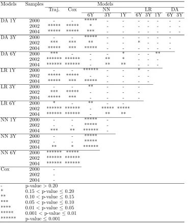
On the whole, discriminant analysis, logistic regression and the neural network are not able to achieve better results than Cox’s method when using multi-period data. Moreover, trajectories and Cox’s method are more resistant than others to changes in economic conditions. They also do significantly better than discriminant analysis and logistic regression, and to a lesser extent, than the neural network. In that sense, they provide a clear gain in stability. To ascertain this fact, we compared the results achieved with all methods and samples from 2000, 2002 and 2004. For this purpose, we carried out a test for differences between the different correct classification rates. The significance levels of this test are shown in Table 6.
Symbols in Table 6 clearly show that the differences between correct classification rates achieved with trajectories and Cox’s method on one hand, and discriminant analysis and logistic regression, on the other, are almost all statistically significant (at the conventional threshold of 5%) when changes in economic conditions occur between the period during which models are estimated and during which they are used for forecasts. But when the p-values exceed this threshold of 5%, they always remain below 10%. Conversely, these differences are not all significant when correct classification rates achieved with trajectories and Cox’s method are compared to those achieved with the neural network. If the comparison is done with six-year period models designed with the neural network, the differences are largely significant. If the same comparison is done with one- and three-year period models, there is no statistical difference with data from 2000 and 2002, whereas the differences are slightly significant with data from 2004 (p-values range from 5% to 20%). We can speculate that the gap between the performances of the different models is the result of the fit between time-series data and the characteristics of the methods themselves since multi-period models designed with conventional methods are much more sensitive to changes in economic con-ditions than trajectories and Cox’s model are. It is worth noting that the neural network performs relatively well with short time-period data (one and three years).
4 5 6 7 8 9 10 11 12 13 14 15 16 17 18 19 20 21 22 23 24 25 26 27 28 29 30 31 32 33 34 35 36 37 38 39 40 41 42 43 44 45 46 47 48 49 50 51 52 53 54 55 56 57 58 59 60 61
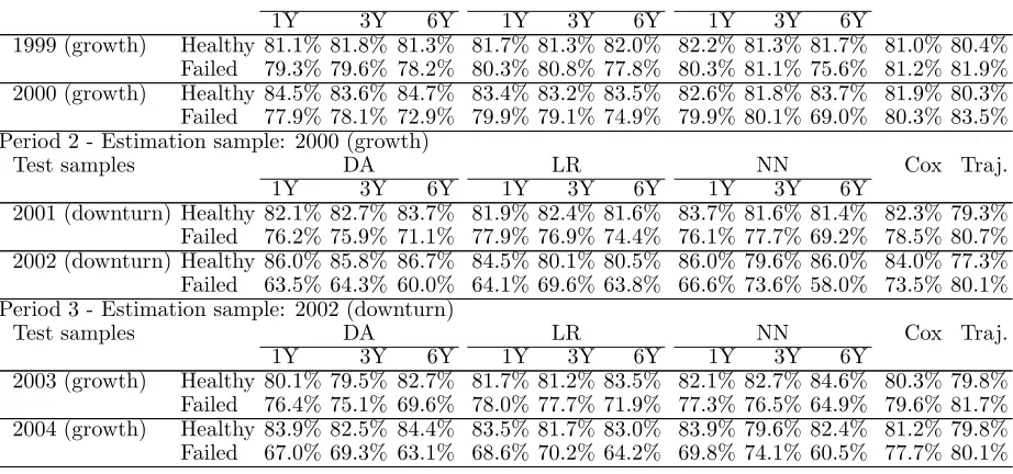
achieve correct classification rates ranging from 80.4% to 82.2% with data from 1999, as opposed to rates ranging from 80.3% to 84.7% with data from 2000. At the same time, failed companies achieve rates ranging from 75.6% to 81.9% and from 69% to 83.5% respectively. And the gap widens greatly with the collection of estimation data during a period of growth, as with the collection of test data during a downturn. In such circumstances, healthy companies achieve correct classification rates ranging from 79.3% to 83.7% with a sample from 2001 and from 77.3% to 86.7% with a sample from 2002. Conversely, for failed companies the figures range from 69.2% to 80.7% with a sample from 2001, and from 58% to 80.1% with a sample from 2002. Figures for classification rates achieved with data from the third period are between those of periods 1 and 2.
This result is consistent with the results of Pompe and Bilderbeek (2005), who noticed that any change in the economic environment makes it more difficult to predict the fate of failed firms than that of healthy firms. Indeed, they found that the moment in which a model’s performance deteri-orates coincided precisely with the moment in which an economic decline and a significant increase in the number of bankruptcies occur. One possible explanation for this phenomenon is that some firms that could have survived in a sound economic climate are no longer able to do so when the climate deteriorates. This reasoning also applies in the opposite situation, as shown in Table 7, with data collected over the third period. Indeed, a model that is designed during a period of downturn and used during a period of growth also fails to accurately forecast the fate of unsound companies.
Table 7 also shows how Cox’s model, and especially trajectories, managed to do better than other methods at predicting the fate of failed firms. Besides, trajectories tend to predict the fate of unsound companies better than that of sound firms. Indeed, with a sample from 2002, correct clas-sification rates of failed (healthy) companies achieved with trajectories are 80.1% (77.3%), compared to rates ranging from 58% to 73.5% (79.6% to 86.7%) for other models. Similarly, with a sample from 2004, figures are 80.1% (79.8%) for trajectories, as opposed to figures ranging from 60.5% to 77.7% (79.6% to 84.4%) for other models.
With multi-period models, the difference between correct classification rates of failed and healthy firms tends to increase compared to that of mono-period models, except with the neural network using three-year period data. In such circumstances, the neural network achieves a correct classifi-cation rate of failed companies that is on average lower than that achieved with Cox’s model (and of course with trajectories), but far better than that achieved with all other models.
4 5 6 7 8 9 10 11 12 13 14 15 16 17 18 19 20 21 22 23 24 25 26 27 28 29 30 31 32 33 34 35 36 37 38 39 40 41 42 43 44 45 46 47 48 49 50 51 52 53 54 55 56 57 58 59 60 61
shown in Tables 8 and 9. These tables show that, in most cases, trajectories do significantly better than other models when predicting the fate of failed companies. It also shows that Cox’s model behaves in a similar manner as trajectories, although it is not as accurate as trajectories, especially when it comes to failed firms. Finally, it points out that the neural network using three-year period data presents some similarities with Cox’s model. Indeed, this model has the ability to better forecast the fate of failed firms than other models do, even if its global accuracy is weaker than that of Cox’s model.
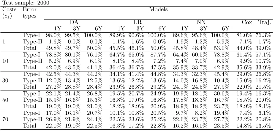
To deepen the results estimated with a cut-off value maximizing the overall classification rate, we analysed how models behave using different misclassification costs. As mentioned in section 3.4.7., the cost of misclassification of healthy firms (i.e., c2) was kept to 1, while the costs of
misclassi-fication of unsound firms (i.e., c1) were respectively set to 1, 10, 20, 30, 40, 50, 60 and 70. The
prior probabilities of the failed and non-failed groups were fixed at 2% and 98%, respectively. The situation where the prior probability of bankruptcy is set to 2%, and the respective costs of mis-classification of healthy and failed firms are set to 1 and 50, leads to mis-classification results that are nearly equal to those obtained when the prior probability of bankruptcy is 50% and when the costs of misclassification are equal and set to 1.
For each period, we calculated the percentage of misclassified companies by model. In order not to overburden the presentation with excessive detail, only misclassification rates achieved with cost 1, 10, 30, 50 and 70 are presented. Tables 10, 11 and 12 show the percentage of misclassified compa-nies by period and by model for different misclassification costs. These tables show that when the classification cost of failed firms is low, trajectories achieve an overall error rate lower than that achieved with all other models. As the cost increases, the errors achieved with all models tend to decrease faster than the error achieved with trajectories, but in nearly all situations this latter error remains the lowest. With data from 2000, all models (except Cox’s model and trajectories) achieve an error ranging from 45.5% to 53% for cost 1, and from 16% to 23.5% for cost 70, whereas trajectories achieve an error of 39% for cost 1 and 13.5% for cost 70. With data from 2002 and all models (except Cox’s model and trajectories), figures range from 41% to 45.6% for cost 1, and from 19.1% to 27.3% for cost 70; and with trajectories, figures are 29.2% for cost 1, and 17.5% for cost 70. With data from 2004, the situation is the same: all models (except Cox’s model and trajectories) achieve an error ranging from 46.4% to 53% for cost 1, and from 22.3% to 26.5% for cost 70; and trajectories achieve an error of 33.3% for cost 1 and 19.7% for cost 70.
4 5 6 7 8 9 10 11 12 13 14 15 16 17 18 19 20 21 22 23 24 25 26 27 28 29 30 31 32 33 34 35 36 37 38 39 40 41 42 43 44 45 46 47 48 49 50 51 52 53 54 55 56 57 58 59 60 61
costs and whatever the period. Only once, with data from 2002, when the cost is equal to 50, does Cox’s model perform better than trajectories. In a few cases (data from 2000 with cost 10 and cost 50; data from 2002 with cost 70), the neural network using three-year period data achieves error rates lower than those obtained with Cox’s model.
As far as misclassification rates of failed and non-failed firms are concerned, when the cost of mis-classification of failed firms is low, all type-II errors are, on average, very low: with data from 2000, type-II errors range from 0% to 7.1%; with data from 2002, figures range from 1.8% to 10.3%; and with data from 2004, they range from 2.9% to 11.1%. By contrast, with data from 2000, trajectories and Cox’s model achieve a type-I error of 76.3% and 81% respectively, compared to type-I errors ranging from 89.6% to 100% with the other models. With data from 2002, for trajectories and Cox’s model figures are 67.5% and 83% respectively, and for other models they range from 94% to 100%. Finally, with data from 2004, figures for trajectories and Cox’s model are 66.8% and 87%, respectively, otherwise they range from 93.0% to 100%.
When the cost increases, trajectories managed to achieve type-I errors that remain far lower than those obtained with other models in any situation. Cox’s model also performed well in terms of type-I errors compared to discriminant analysis, logistic regression and the neural network, even if the neural network using three-year period data outperformed Cox’s model in a few situations (data from 2000 and costs 10 and 50, data from 2002 and cost 70).
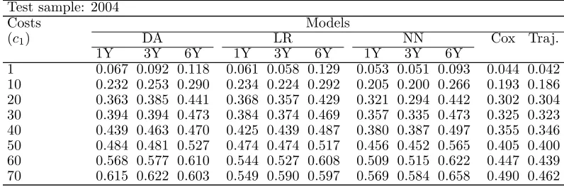
Based on the results used to calculate Tables 10, 11 and 12, we have assessed the resubstitution risks of each model for all costs of misclassification. Tables 13, 14 and 15 show the resubstitution risks of all models assessed with data from 2000, 2002 and 2004.
In these three tables, the comparison of trajectories with other models for costs ranging from 1 to 70 shows that trajectories slightly dominate Cox’s model, and all other models substantially. In Table 13, trajectories dominate all models in terms of resubstitution risks for all but costs 1 and 10. In Table 14, aside from Cox’s model for cost 50, trajectories also dominate all models. And in Table 15, trajectories continue to dominate all models. We must add that, for cost 20 that is not presented in Table 15, Cox’s model and the neural network using three-year period data have a lower overall cost than that of trajectories. We can also observe that Cox’s model, especially with data from 2002 and 2004, slightly dominates the neural network using one- and three-year period models.
4 5 6 7 8 9 10 11 12 13 14 15 16 17 18 19 20 21 22 23 24 25 26 27 28 29 30 31 32 33 34 35 36 37 38 39 40 41 42 43 44 45 46 47 48 49 50 51 52 53 54 55 56 57 58 59 60 61
one- and three-year period data. These models are more robust to any changes in the misclassifica-tion costs than the others. Then, the second group is made up of one- and three-year period models designed with discriminant analysis and logistic regression. The third and last group is made up of six-year period models.
The results we obtain with conventional modelling techniques of designing financial failure models are consistent with the results of many studies published in the literature. Firstly, the assumption that model prediction ability depends on data stationarity is validated: model accuracy is indeed dependent on the phase of the business cycle during which data collection occurs. Secondly, changes in economic conditions involve asymmetric effects on model accuracy depending on whether com-panies are healthy or if they have failed; forecasting the fate of failed comcom-panies becomes even more difficult as the magnitude of changes increases.
The results we obtain with trajectories show that, when company status (healthy vs. failed) is not taken into account, and if the economic environment remains stable, their performance is similar to that achieved with other models. However, if the economic environment changes, then trajectories achieved similar results to those achieved with Cox’s model, but better than those achieved with other models. But, when company status is taken into account, model performance depends heavily on this status. When it comes to predicting the fate of unsound firms, trajectories are indeed less sensitive to economic changes than other models are. If changes are slight, trajectories perform as well as Cox’s model or the neural network using three-year period data (see Table 7), but better than the other models. And if changes are great, type-I error (misclassifying a failed firm) is much lower than that achieved with all other models, and this result also holds when misclassification costs are taken into account – a point that is particularly important. With equal performance, a good model is a model able to minimize type-I error because, as we have noted, the cost of this error is far greater than that of a type-II error (misclassifying a healthy company). Moreover, when it comes to predicting the fate of healthy companies, trajectories perform slightly worse than other models.
5. Conclusion
4 5 6 7 8 9 10 11 12 13 14 15 16 17 18 19 20 21 22 23 24 25 26 27 28 29 30 31 32 33 34 35 36 37 38 39 40 41 42 43 44 45 46 47 48 49 50 51 52 53 54 55 56 57 58 59 60 61
on how to stabilize model accuracy over time.
Our results confirm that the accuracy of conventional models is closely related to changes that occur in firms’ economic environment over the period during which models are estimated and used to do forecasting. Their accuracy is even worse when the growth differential between the model estimation period and the test period is large, whereas trajectories achieve much more stable results. Moreover, when model accuracy deteriorates, the error made with conventional models is caused mainly by a sharp fall in type-I error, whereas trajectories achieve rather well-balanced results for type-I and type-II errors.
Trajectories can therefore increase the reliability of failure models over time and reduce the cost of errors in decision-making that may occur in financial institutions. They can also help settle the issue about the time intervals beyond which a model must be re-estimated. However, the novelty of this method is also its weakness. The results obtained in this study require confirmation with other samples and other types of firms. But, beyond this issue, other uses of trajectories might be explored. For one thing, they can be used as a diagnostic tool, to assess a company’s financial situation, as Sueyoshi and Goto (2009) suggested a revamped version of Altman’s (1968) z-score for a similar use. Therefore, one should analyse their informational content with regard to that of other diagnostic methods. For another, they might be used to tackling conceptual issues – for example, how to better understand some financial behaviours that characterize firms, whether they are healthy or not. It would be valuable to study what this representation might bring to the understanding of the bankruptcy process itself.
Acknowledgment
We are very grateful to the three anonymous reviewers for their substantial contribution to the improvement of this article.
References
Agarwall, V., Taffler, R. J., 2007. Twenty-five years of the Taffler z-score model: Does it really
have predictive ability? Accounting and Business Research 37, 285–300.