http://www.scirp.org/journal/jst ISSN Online: 2161-1238
ISSN Print: 2161-122X
Exponential Stabilization and Estimation for
Sampled Observer Design of Surface Mounted
Permanent Magnet Synchronous Motor
A. A. R. Al-Tahir
Electrical Engineering Department, University of Kerbala, Kerbala, Iraq
Abstract
A nonlinear state observer design with sampled and delayed output measurements for variable speed and external load torque estimations of SPMSM drive system has been addressed, successfully. Sampled output state predictor is re-initialized at each sampling instant and remains continuous between two sampling instants. Through-out this study, a positive constant to satisfy an upper limit of the sampling period between sampling instants and allowable timing delay in terms of observer parame-ters has been prepared such that the exponential stable of the closed-loop system is guaranteed, based on Lyapunov stability tools. In order to validate the theoretical results introduced by main fundamental theorem to prove the observer convergence, the proposed sampled-data observer is demonstrated through a sample study appli-cation to variable speed SPMSM drive system.
Keywords
Stability, SPMSM, Sampled Output Observer, Lyapunov Stability, Intelligent Sensor
1. Introduction
In recent decays, synchronous machines are used in variable speed motoring and the manufacturers had been made synchronous machines based on permanent magnets in wide power range with various categories and structures. On the other hand, an effi-cient development has been considered in the field of power electronics technology; it has made the task of flexible rotor speed variation a realizable target. In effect, PMSMs are more efficient for applications demanding rotor speed reversion. Synchronous ma-chine is convenient for drive applications, when these applications involve wide power
How to cite this paper: Al-Tahir, A.A.R. (2016) Exponential Stabilization and Esti-mation for Sampled Observer Design of Surface Mounted Permanent Magnet Syn-chronous Motor. Journal of Sensor Tech-nology, 6, 122-140.
http://dx.doi.org/10.4236/jst.2016.64010
Received: October 2, 2016 Accepted: November 21, 2016 Published: November 24, 2016
Copyright © 2016 by author and Scientific Research Publishing Inc. This work is licensed under the Creative Commons Attribution International License (CC BY 4.0).
http://creativecommons.org/licenses/by/4.0/
variation. To this end, PMSMs have been made controllable through inverters since these inverters have the possibility of interconnection between electrical grid and three-phase machines and they are capable to ensure smooth output voltage. The latter allow the control of stator phases switching action, depending on the electrical rotor position, so that the PMS motors operate with time-varying speed. The inverters are acted on using controllers, but these need online measurements of the rotor speed and load torque [1]. The point is that mechanical sensors are costly and may not be suffi-ciently reliable. Accordingly, state observers have been reported in recent years to get online estimates of mechanical variables based on on-line measurements of the elec-trical variables. Various design approaches had been used to obtain mechanical sense-less observers for PMSMs. One of the design approaches dealing with the identification and investigation of eddy current effects on motor rotor position observation had been claimed by [2]. The authors tried to improve high frequency injection approach based on self-sensing control of a PMSM drive system at stand still and low rotor speed. This approach is not recommended for high rotor speed applications and LFI. On the other hand, some of excitation strategies had been recommended by [3] that rely on the de-tection of the rotor position from the stator voltages and currents without requiring additional test signals. In [4], the back EMF (waveform of the voltage induced in stator windings) had been used to estimate rotor position by means of state observers or Kal-man filters [5]. This approach works well in medium and high speed applications, but it is not accurate at low operation when the back EMF is low. In [6], Kalman-like inter-connected observers have been designed that estimate the machine position and speed. However, these observers are complex (computation time consuming), and their con-vergence analysis relies on an excitation condition involving the observer signals (e.g. the state estimates). More specifically, an interconnected observer is in fact composed of two observers and the persistent excitation condition of one observer involves the state estimates provided by the other. As a matter of fact, suitable conditions are those involving the system signals (system input and output) not the observer signals.
Recently, the problem of global exponential stabilization of nonlinear systems has received a great deal attention in the world. Consequently, this paper deals with de-signing of nonlinear sampled-data observers in the presence of sensorless measure-ments, all the mechanical state variables are considered inaccessible for measurements. As investigated in [7] [8], some extra growth conditions on the unmeasurable states of the system are usually necessary for the global stabilization of nonlinear time delay sys-tems. A Lyapunov-Krasovskii Functional (LKF) was suggested in [9], such that the rela-tion between the delayed state variable and the number of cascade observers with spe-cific vector gain were introduced. In [10] [11] claimed that several authors extended the result in [9] to a time-varying delay system with observer and provided a maximum al-lowable time delay in terms of observer design parameters.
me-thods.
Sufficient conditions for time-varying delays were derived via Razumikhin approach
[13], which leads to more conservative results than Krasovskii method. For systems with constant delays, sufficient conditions were derived in terms of LKF in [14]. Pub-lished studies concerning with the design of continuous-time high-gain observers [15] [16] dealing with dynamical high-gain observers for continuous-time systems are de-signed.
In present paper, one looks for accurate observation of the unmeasured mechanical state variables, which are angular rotated speed and external load torque for surface permanent magnet synchronous motor SPMSM, supposing the stator current and vol-tage to be accessible for measurements. To this end, a sampled-data nonlinear state ob-server will be designed with sampled and delayed output measurements coupled with inter-sampled output state prediction. The proposed observer will prove to be expo-nentially convergent in presence of wide range variations. The proposed observer is ca-pable to ensure efficient tracking response. The proposed observer is formally proved through a main result based on tools of Lyapunov stability approach.
The remainder of this paper is organized as follows. In the next section, the problem formulation of SPMSM will be provided. The Third section is devoted to the observer design and stability analysis with sampled and delayed measurements is provided by using a Lyapunov stability approach. Then the equations of the state observer used for SPMSM are given. In this section, the problem statement which leads us to prove the exponential convergence of the global exponential stabilization and state estimation of nonlinear systems coupled with sampled–data observer design based on main theorem. The forth section is simulation results and verifications. Finally, conclusions are given in section five.
2. Problem Formulation
2.1. Reduced Model of SPMSM
Dynamic modelling is needed for various types of analysis related to system dynamics: stability, control system, and optimization. The SPMSM model is constructed in (α β− ) stationary reference frame. Notice that, the time derivative of the external
in-put load torque is considered by an unknown bounded function
( )
t . The controlob-jective is to determine under what sufficient conditions that all the SPMSM states va-riables, which are, ψ ωr r and TL can be determined from the motor input and output
measurements, namely the stator current and the motor input command voltage signal,
s
i and us.
(
)
( )
d 1 d ? d 1 d ? d d d d 1.5 d 1 d d d p s ss r r s
s s s
p
s s
s r r s
s s s
r
p r r
r
p r r
p v
r
r s r s r L
L
n
i R
i u
t L L L
n
i R
i u
t L L L
n t model n t n f
i i T
t J J J
T t t
α
α β α
β
β α β
α
β
β
α
α β β α
ω ψ
ω ψ
ψ ω ψ
ψ
ω ψ
ω ψ ψ ω
= − + + = − − + = − Σ = = − − − = (1)
with, def
(
)
s s s
i =col iα iβ , ψrdef=col
(
ψrα ψrβ)
,(
)
defs s s
u =col uα uβ are respectively,
the stator vector of currents, the rotor fluxes and the motor input command signals.
r
ω and TL respectively, denote the rotor speed and the load torque, which is unknown
but constant and that its upper bound is available. J and fv are the moment of inertia
and viscous friction; np is the number of magnetic pole pairs. The electrical
parame-ters, Rs and Ls are the armature resistor and inductance, respectively. The
electromag-netic torque, Tem, is indirect measurable output state. This can be evaluated through
the first term of third subsystem given in (1). One can write the system under study of SPMSM as:
(
)
(
)
( )
1 , , 2 ,
1
em s s r s r r
em v
r r L
L
T i u i
T f
T
J J J
T t
γ ψ γ ψ ω
ω ω = − = − − = (2)
where
(
(
)
)
(
)
(
)
(
)
(
)
1
2 2 2 2
1.5 , , . , 1 1.5 p
r s r s s r s r s s
s s r
s r
p r s r s r r
s n
u u R i i
L i u
i
n i i
L
α α β β α β β α
α α β β α β
ψ ψ ψ ψ
γ ψ
γ ψ
ψ ψ ψ ψ
− − − + + +
This model can be re-written under the form taking into account that the electro-magnetic torque Tem
( )
t is not accessible to measurement all the time, only sampled–data measurements, Tem
( ) (
tk , k=0,1, 2,)
are available:(
)
(
)
( )
( )
1( )
( )
, ,
s r s
k k k em k
x F i x G x u
y t Cx t x t T t
ψ
= + + Σ
= = = (3)
where, the state vector def
(
)
def(
)
1, 2, 3 em, r, L x=col x x x =col T ω T(
)
(
)
2
0 , 0
1
, 0 0
0 0 0
s r s r i F i J γ ψ ψ − − ,
(
)
(
)
1 3 1 2 , , , 0s s r
v s
i u
f x
G x u x
J J γ ψ − ∈
, and
0 0
Σ
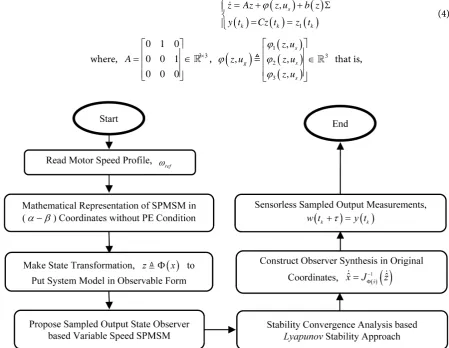
To clarify the general procedure related with this study, a flow block diagram of study method and its application to sensorless SPMSM drive system is shown in Figure 1.
2.2. System Construction in z Benchmark
Let us provide the following state transformation to put the system model in observable normal form as follows:
3 3
Ф : →, us us def
( )
xx z
= Φ
such that,
( )
(
)
(
)
1
3
2 2
2
3 , , g r
g r x
z x i x
i x J
γ ψ
γ ψ
Φ = − ∈
is diffeomorphism.
Let us put the following system in the z benchmark after doing state transformation is:
(
) ( )
( )
( )
1( )
, s
k k k
z Az z u b z
y t Cz t z t
ϕ
= + + Σ
= =
(4)
where, 3 3
0 1 0
0 0 1
0 0 0
A ×
= ∈
,
(
)
(
)
(
)
(
)
1
3 2
3
,
, ,
, s
g s
s
z u
z u z u
z u
ϕ
ϕ ϕ
ϕ
∈
[image:5.595.102.552.335.683.2] that is,
(
)
(
)
(
) ( )
1 2 1
2 3 2
3 3 , , , s s s
z z z u
z z z u
z z u b z
ϕ ϕ ϕ = + = +
= + Σ
(5)
where,
(
)
(
)
1 1
2 2 2
2 3 3 , , em s r s r
z x T
z i x
i z x J γ ψ γ ψ = = = − = and,
(
)
(
)
(
)
(
)
1 1 1.5, s s, s, r p r s r s s r s r s
s
n
z u i u u u R i i
L α α β β α β β α
ϕ =γ ψ = ψ −ψ − ψ −ψ
(
)
(
)
(
)
{
(
)
(
)
(
)
2 2
2 1 2 2 2 2
2 2 2 2 2 3 2 ,
, , 1.5
1
3 1
s r v
s s r p r s
p s
r s r r s p r s
s s s
p s
r s r s r r
s s s
p
s
i f
z u x i x x p n x i
J J
n R
i u n x i
L L L
n n
R
i x u x x
L L L L
β α
α α β α α β
β β α β β α
γ ψ
ϕ γ ψ ψ
ψ ω ψ ψ
ψ ψ ψ ψ
− = + − − − − + + − + − + − − + − +
(6)
(
)
(
)
(
)
(
)
2 3
3 2 2
3
2 2
2 2 2
1
, 1.5
3 1
p
s p p r s r r s
s s
p p
p r s r r s r r
s s s
n x
z u n n x i x u
J L L
n n
n x i x u x
L L L
β α α β α
α β β α β β α
ϕ ψ ψ ψ
ψ ψ ψ ψ ψ
= − − + − + − + + − + With
( )
2(
)
1 , s r
b z i
Jγ ψ
= (7) Before the observer synthesis for our physical system model given in (4) is designed, some technical assumptions have to be stated. Such hypothesis have vital role for the next results.
H1: The functions, ϕi
(
z u, s)
: n× n→n are locally Lipschitz and globallybounded with respect to z in domain of interest, uniformly in ug i.e., ∃β0>0, such
that,
( )
,ˆ n n, , sz z u U
∀ ∈ × ∀ ∈ we can easily write the following:
(
ˆ, s)
(
, s)
0 zf z u − f z u ≤β e (8)
Note that the functions ϕi
(
z u, s)
may contain linear parts and the dynamics zndepends on all state variables z1,,zn through the Lipchitz function ϕ
(
z u, s)
.H2: Throughout this paper the function Σ
( )
t is unknown periodic bounded andthe real δ >0 is the upper bound of Σ
( )
t <δ such that, b z T( )
L ≤β δ β1 ,∃ >1 0.Lemma [18]: Let us consider that the input us is regularly persistent for system
given in (4) and assuming the Lyapunov differential equation stated in (10), ∃ >θ0 0
so that for any symmetric positive definite matrix S(0), ∀ >µ µ0, ∃ >α 0,β>0,t0 >0
such that ∀ ≥t t0,αIn ≤S t
( )
≤βIn. Also, by choosing µ0>2ς, one has2
1exp .
3. Observer Structure
In this subsection, the following sampled-data observer is proposed for k∈ ,
[
k ,k 1)
t t τ t+ τ
∀ ∈ + + . The main difference compared with third class of nonlinear sys-tem given in [19] resides in the presentation of state observer with the effect of external disturbance. As a matter of fact, the authors in [20] focused in case of linear systems and without taken into consideration the state predictor.
(
)
1 T(
(
)
( )
)
0ˆ ˆ, ˆ
ˆ g
z=Az+ϕ z u −S C− Cz t−τ −w t (9)
T T
S= −θS−SA−A S+C C (10)
(
)
0(
(
) (
)
)
ˆ ˆ , g
w=CAz t−τ +Cϕ z t−τ u t−τ (11)
(
k)
( )
kw t +τ =y t (12)
The output sampled data observer defined from (9)-(12) consists of a classical observer and output predictor for sampled and delayed measurements where 3
ˆ
z∈ is the
continuous estimates of the states. The predictor w is reset (re-initialized) at each sam-pling instant. S is SPD matrix and continuous in +,S
( )
0 >0. Now, one shall provein the next theorem that the proposed observer is a global exponential observer for sys-tem given in (4) with the sampled and delayed measurements in output state vector,
[
1)
, k , k
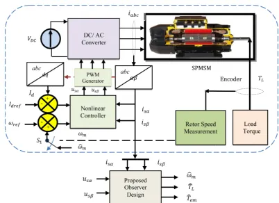
k∈ ∀ ∈t t +τ t + +τ , where is set of natural numbers. Figure 2 shows single
[image:7.595.148.551.389.681.2]line diagram of proposed study with sampled and time delayed state observer.
Theorem (Main Result): Let us consider the system described by the set of differen-tial equation given by (4), and hypothesis H1, H2 hold. This leads us for constant
max-imum allowable sampling period TMASP and upper bound limit of admissible timing
delay τMATD in output state measurements as follows:
( )
0 2 1 m MASP m m T Cb zCA Cβ
α α
Θ ≥
+ + Θ + + Θ
(13) and, min 2
1 1 0 1
1
min , ,
2 2 2 2
MATD
m m m
T
C C CA
α τ
α α β α
<
Θ + Θ + + Θ +
m
m
(14)The sampled output-data observer given in Equations (9)-(12) is global exponential observer for system (4) as t→ ∞ for sufficient large positive value of observer design
parameter, satisfying, θ>1.
Proof of theorem: The searcher shall give formal analysis of the main theorem using Lyapunov stability approach. For writing convenience, the variable t can be cancelled. Set observation error: def
ˆ z
e = −z z, then one shall obtain from Equations (9)-(12) and (4)
the following new dynamics error system as follows:
( ) ( )
( )
1 T(
(
)
)
,
ˆ, ˆ
z z o g g
e =Ae +ϕ z u −ϕ z u −b z Σ −S C− Cz t−τ −w (15)
Throughout this paper, let us define the following quantities:
(
)
def w
e = −w y t−τ (16)
(
)
def(
) (
)
ˆ, , g o ˆ, g , g
z z u z u z u
ϕ =ϕ −ϕ (17)
Thanks to Newton Leibniz integration formula that it will be used in next equations:
(
)
t( )
dz z t z
e t−τ =e −
∫
−τe ξ ξ (18)Then the error dynamics given by (15) can be re-formulated as:
(
1 T)
(
)
( )
( )
1 T , ,ˆ t d
z z g t z w
e A S C C e z z u b z e S C e
τ
ϕ ξ ξ
− −
−
= − + − Σ +
∫
+ (19)
Let us define the following LKF, provided by [20]:
( )
( )
2T
d d t t
z z t z w
W=e Se +
∫ ∫
−τ σ e σ ϑ+ Θ t edef
1 2 3
W =V +V +V (20)
where ϑ>1 is a positive design parameter and Θ
( )
t is a piecewise differentiablepositive function designed for the purpose of correcting the error between the predictor and the output such that, Θ
( )
t satisfies the following conditions:( )
( )
( )
[
1)
0, 0
,
0, , ,
k m
k k
t t
t k
t k t t t
+
+
Θ > ∀ > Θ = Θ ∈ ∈
Θ < ∈ ∀ ∈
To show the exponential convergence of the observation error, it is necessary to pre-pare conditions for TMASP and TMATD to guarantee that:
[
1)
, k , k
W ≤ −hW ∀ ∈t t +τ t + +τ (22)
(
k)
(
k)
,W t +τ ≤W− t +τ ∀ ∈k (23)
Using the fact that the observation error ez is continuous and the error
(
)
0,w k
e t +τ = then it is clear that the inequality defined in (22) is performed.
Now, let us decomposes the Lyapunov function into four functions, which are V V1, 2
and V3, respectively:
( )
( )
def T 1 def 2 2 def 3 d d z z t t z t wV e Se
V e
V t e
τ σ σ
ϑ − = = = Θ
∫ ∫
(24)Now, the time derivative of the first Lyapunov function is:
T T
1 z z 2 z z
V =e Se + e Se (25)
Combining (10) and (19) for S and ez, respectively, yields
( )
(
)
T T T T T
1 2 d
t
z z z z z t z w
V e Se e C Ce e C C e e
τ
θ ξ ξ
−
= − − +
∫
+ (26)
Using the fact that,
( )
(
)
( )
2T T T T
2 z t z d w z z t z d w
t t
e C C e e e C Ce C e e
τ ξ ξ τ ξ ξ
− + ≤ + − +
∫
∫
This will give,
( )
2 22 T
1 2 d 2
t
z z t z w
V e Se C e e
τ
θ ξ ξ
−
⋅
≤ − +
∫
+ (27)
Thanks to Jensen’s inequality, one has:
( )
2( )
2d d
t t
z z
t−τe ξ ξ ≤τ t−τ e ξ ξ
∫
∫
(28)This leads us to get the following result,
( )
2 22 T
1 2 d 2
t
z z t z w
V ≤ −θe Se + τ C
∫
−τ e ξ ξ+ e (29)In view of Lemma, one deduce T 2
z z z
e Se e
θ θα
− ≤ −
( )
2 22 2
1 2 d 2
t
z t z w
V ≤ −θα e + τ C
∫
−τ e ξ ξ+ e (30)And, the time derivative of V2 given in (30) is:
( )
2 2
2 d
t z t z
V =τ e −
∫
−τ e ξ ξ (31)On the other hand from (9)-(12), one can easily conclude that:
( )
22
2 2
0
d ,
t
z z w t z
e ≤ e + e + −τ e ξ ξ ∈ +
∫
That is, the system (31) becomes:
( )
2( )
2 2 2 2 d d t t
z w t z t z
V e e e e
τ τ
τ − ξ ξ − ξ ξ
= + +
∫
−∫
m
(33)Likewise, the time derivative of third Lyapunov function in (24) is:
( )
( )
3
2
2 w w w
V = ϑΘ t e e + Θϑ t e (34)
The time derivative of the prediction error given in (16) is:
( )
(
)
w
e =w t −y t −τ (35)
Using (11) and (29) with the assistance of the Newton Leibniz integration formula stated in (18) and using H2, one gets:
(
ˆ, ,)
( )
( )
d 0( )
dt t
w z g t z t z
e C Ae z z u b z C A e e
τ τ
ϕ − ξ ξ β − ξ ξ
= + − Σ − +
∫
∫
(36)
Since,
( )
d 0( )
d( )
t t
w z t z t z
e CA e e C e Cb z
τ ξ ξ β τ ξ ξ
− −
≤ ⋅ + + + Σ
∫
∫
Therefore, the first term of (34) becomes:
( )
( )
( )
( )
( )
( )
2 2 2 2 0 2 2 2 2 d d d tw w w z t z
t
w z t z
t
w w t
t e e t CA e e e
C e e e
e Cb z e
τ
τ
τ
ϑ ϑ ξ ξ
β ξ ξ
δ ξ ξ
−
−
−
Θ ⋅ ≤ Θ + +
+ + +
+ + + + Σ
∫
∫
∫
(37)Using once again Jenson’s inequality given in (28), and using, H3, yields:
( )
( )
{
( )
( )
2 2 2 2 02 2 2 d
2 2 d
t
w w w z t z
t
w z t z
t e e t CA e e e
C e e e
τ
τ
ϑ ϑ τ ξ ξ
β τ ξ ξ
−
−
Θ ≤ Θ + +
+ + +
∫
∫
(38)
So, combining Equation (38) in (34), one has:
( )
{
( )
( )
( )
2 2 3 2 2 2 02 2 d
2 2 d
t
w z t z
t
w z t z w
t CA e e e
C e e e
V
t e
τ
τ
ϑ τ ξ ξ
β τ ξ ξ ϑ
−
−
≤ Θ + +
+ + + + Θ
∫
∫
(39)
Thus, from equations (30), (31) and (39), one has the following
( )
( )
( )
( )
( )
( )
( )
( )
( )
2 0 2 0 2 2 2 02 2 2
2
2 1 2 2 d
z
w
t z t
W t C e
CA t Cb z C t t e
C CA t C t e Cb z
τ
θα τ ϑ β
τ ϑ β ϑ ϑ
τ τ τ ϑ τ β ϑ ξ ξ δ
−
≤ − − Θ − +
+ + + Θ + + Θ + Θ
+ + − + Θ + Θ
∫
+
m
m
m
(40) Thus, the exponential convergence of the observation error is guaranteed if the fol-lowing conditions successfully achieved:( )
( )
0( )
2 t 2 t C 2 2 CA t h 0
( )
( )
0( )
( )
2+τ
m
+ CAϑΘ t + Cb z + Cβ ϑΘ t + Θϑ t +hϑΘ ≤m 0 (42)( )
( )
2
0
2τ C +τ
m
− +1 2τ CAϑΘ t +2τ β ϑC Θ t +hτ≤0 (43)To derive the, TMASP and TMATD, let us consider h 0
+
→ , τm≤α and, ϑ α= ,
this implies, (41) becomes:
( )
( )
0( )
2 t 2 t C 2 2 CA t
θα≥ τ ϑ
m
Θ + ϑΘ β − ϑ− ϑΘ0
2 m 2 m C 2 2CA m
θ≥ αΘ + Θ β − − Θ (44) Furthermore, one selects the function Θ
( )
t as a saw tooth function for, k∈,0
+
∈
, Θ
( )
tk = Θ ∈m ,( )
t+
Θ < − ∈ , and T >0. Consequently, the proposed
condition in (42) is performed if,
( )
20 2 2
1
4 2
1
exp
m m T
Cb z C
CA Cβ τ µ
α α α −
= + + Θ + + Θ +
(45)
This leads us that the sampling interval must be smaller than TMASP, t 0
+
∀ ∈ ,
( )
t 0Θ > . Using (45), the proposed maximum admissible sampling interval is:
( )
20 2 2
1
4 2
1
exp m
MASP
m m T
T
Cb z C
CA Cβ τ µ
α α α −
Θ ≥
+ + Θ + + Θ +
(46)
On other hand, from condition (43), the corresponding admissible timing delay,
MATD
τ is
min 2
2
1 1 0 1 2
1 1
min , ,
4
2 2 2 2
exp MATD
m m m T
T
C
C C CA µ
α τ
α α β α
α −
<
Θ + Θ + + Θ + +
m
m
(47) It is obvious that if Equations (45), (46) and (47) are performed successfully, the proposed conditions given in Equations (41), (42), (43) and (44) are satisfied in the same way. Thus the observation error of the system under study tends exponentially towards the origin as the time increasing towards infinity. This ends proof of theorem.
4. Simulation Results
In this section, the dynamic performances of the proposed sampled data observer ac-companied by sampled and delayed output measurements for online estimation of SPMSM state variables, which are motor rotor speed and external load torque. SPMSM has been implemented under MATLAB/Simulink environment. The tool selected for solving the dynamic equations is the MATLAB function called ODE45.
on line estimates of all mechanical state variables in SPMSM. The sampled data observ-er stated in system (9) is implemented using realistic benchmark MATLAB/Simulink resources. The observer design parameters are θ,Ts and τ. The dynamic
perfor-mance depends on the numerical value given to the observer design parameters, con-stant sampling period, Ts between sampling instants and allowable timing delay. The
selection of the tuning parameter θ is performed using try and error procedure. This value has been bounded to 200 as listed in Table 1 when simulating sampled–data non-linear observer given in Equation (9). From Table 1, the electrical time constant is
12.6 ms s s
L R = accordingly, a suitable value of the allowable timing delay would be 6
ms. A time delay of 6 ms appears be sufficient to exceed transient stability. The sum-marized results for sampled-data observer design parameters θ,Ts and τ are listed
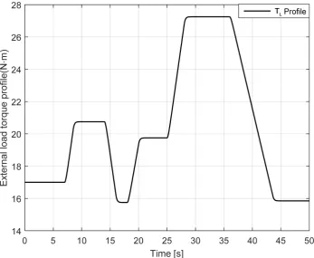
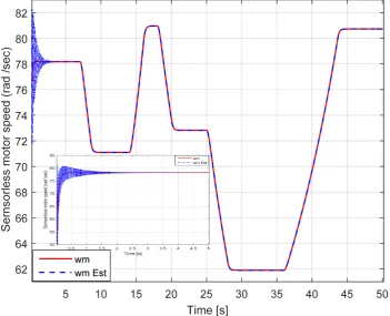
in Table 2. The nonlinear observer dynamic performances for complete one cycle of (50 s). Figure 3 shows reference rotor speed in (rad/sec) to guarantee control strategy.
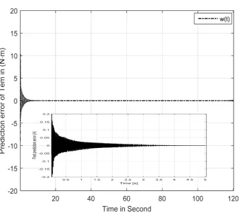
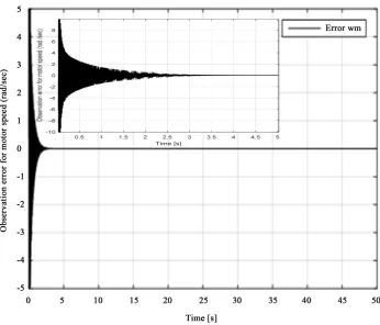
Figure 4 clarifies the external load torque profile in (N∙m). Figure 5 illustrates real electromagnetic torque and its estimates. On the other hand, the rotor speed and load torque tracking performances are shown in Figure 6 and Figure 7, respectively. The output state prediction error is shown in Figure 8. It is apparent that the output elec-tromagnetic torque and its prediction is decreased and increased simultaneously with variation of angular rotated speed. Thus, the observation errors resulting from technical hypothesis H1, H2 are practically acceptable as shown in Figure 9 and Figure 10. It
[image:12.595.196.555.457.608.2]should be mentioned that the dynamic tracking performance of the proposed sampled and delayed observer is quite satisfactory. From these figures, the error dynamics are exponentially convergence to origin and the closed-loop sample study is globally asymptotically stable GAS with time progressive.
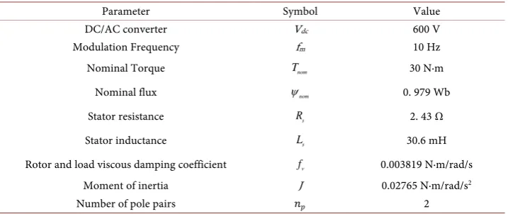
Table 1. Nominal SPMSM characteristics.
Parameter Symbol Value
DC/AC converter Vdc 600 V
Modulation Frequency fm 10 Hz
Nominal Torque Tnom 30 N∙m
Nominal flux ψnom 0. 979 Wb
Stator resistance Rs 2. 43 Ω
Stator inductance Ls 30.6 mH
Rotor and load viscous damping coefficient fv 0.003819 N∙m/rad/s
Moment of inertia J 0.02765 N∙m/rad/s2
[image:12.595.201.553.638.703.2]Number of pole pairs 𝑛𝑛𝑝𝑝 2
Table 2. Values of the observer design parameters.
Index Value
Observer design θ 200
Sampling period Ts 2 ms
Figure 3. Reference speed in (rad/sec).
[image:13.595.200.548.400.685.2]Figure 5. Real Tem and its estimate.
[image:14.595.198.550.397.682.2]Figure 7. Load torque and its estimate.
[image:15.595.200.549.378.689.2]Figure 9. Observation of rotor speed.
The initial conditions of the matrices S t
( )
is set as, S( )
0 =3, where 3∈R3 3× isidentity matrix and S t
( )
is symmetric positive definite matrix and solution of theLyapunov equation. The initial conditions of the system states are chosen:
( ) ( ) ( )
T[
]
T1 0 , 2 0 , 3 0 0, 0,17
x x x =
and the corresponding observer states are chosen
as,
( ) ( ) ( )
T[
]
T1 2 3
ˆ 0 ,ˆ 0 ,ˆ 0 10 15, 0,
x x x =
. A solution of the Lyapunov equation given by
Equation (10) is: 1 T
(
)
1 2 3[
]
3 3 3
! ! ! , , 3, 3,1
S C− =n n−p p =col C C C =col is the binomial
coefficient. The simulations have been achieved successfully with stator inputs in sta-tionary reference frame are, usα =220 sin
( )
π ,t usβ =220 cos( )
π .tThe simulation results for our case study claimed that the proposed sampled-data observer has acceptable transient response, with influence of sampled and delayed out-put measurement, accurate tracking response and robustness of observer performance for unknown mechanical torque.
5. Conclusion
In this study, synthesis of nonlinear hybrid state observer for a class of MIMO systems accompanied by sampled and delayed output measurements has been achieved suc-cessfully. The observer convergence is formally analyzed and clarified by numerical si-mulation of surface mounted PMSM drive system. As already mentioned, mechanical sensors based solutions are most costly and unreliable. Then, state observers turn out to be a quite natural alternative to get estimates of mechanical variables using only mea-surable electrical state variables. The proposed observer provides estimates of the me-chanical state variables (rotor speed, load torque) using stator currents and voltages measurements. The numerical results presented in this paper are interesting and could be practically useful from the view point of engineers. The searcher provided an upper bound of constant sampling period and allowable timing delay with sufficient large value of observer synthesis parameter that will ensure the global exponential conver-gence of the observation and prediction errors towards zero using Lyapunov stability theory.
Acknowledgements
I greatly appreciate the financial support given from ministry of higher education and scientific research in Iraq to carry out this research.
References
[1] Tety, P., Konaté, A., Asseu, O., Soro, E. and Yoboué, P. (2016) An Extended Sliding Mode Observe for Speed, Position and Torque Sensorless Control for PMSM Drive Based Stator Resistance Estimator. Intelligent Control and Automation, 7, 1- 8.
http://dx.doi.org/10.4236/ica.2016.71001
[2] Hu, J.G., Xu, L.Y. and Liu, J.B. (2006) Eddy Current Effects on Rotor Position Estimation for Sensorless Control of PM Synchronous Machine. IEEE Industry Applications Confe-rence,Tampa, 8-12 October 2006, 2034-2039. http://dx.doi.org/10.1109/ias.2006.256815
EKF Estimation of Speed and Rotor Position. IEEE Transactions on Industrial Electronics, 46, 184-191. http://dx.doi.org/10.1109/41.744410
[4] Fakham, H., Djemai, M. and Busawon, K. (2005) Design and Practical Implementation of a Back-EMF Sliding-Mode Observer for a Brushless DC Motor. IET Electric Power Applica-tions, 2, 807-813.
[5] Lang, B., Liu, W. and Luo, G. (2007) A New Observer of Stator Flux Linkage for Permanent magnet Synchronous Motor Based on Kalman Filter. 2nd IEEE Conference on Industrial Electronics and Applications, 1813-1817.
[6] Ezzat, M., Leon, J.D. and Glumineau, A. (2011) Sensorless Speed Control of PMSM via In-terconnected Observer. International Journal of Control, 84, 1926-1943.
http://dx.doi.org/10.1080/00207179.2011.629684
[7] Ahmed-Ali, T., Karafyllis, I. and Lamnabhi-Lagarrigue, F. (2013) Global Exponential Sam-pled-Data Observer for Nonlinear Systems with Delayed Measurements. System and Con-trol Letters, 62, 539-549. http://dx.doi.org/10.1016/j.sysconle.2013.03.008
[8] Karafyllis, I., Krstic, M., Ahmed-Ali, T. and Lamnabhi-Lagarrigue, F. (2014) Global Stabili-zation of Nonlinear Delay Systems with Compact Absorbing Set. International Journal of Control, Taylor & Francis, 8, 1010-1027. http://dx.doi.org/10.1080/00207179.2013.863433
[9] Ahmed-Ali, T., Cherrier, E. and M’Saad, M. (2010) High-Gain Observer for a Class of Time-Delay Nonlinear Systems. International Journal of Control, 83, 273-280.
http://dx.doi.org/10.1080/00207170903141069
[10] Ahmed-Ali, T., Cherrier, E. and Lamnabhi-Lagarrigue, F. (2012) Cascade High-Gain Pre-dictors for a Class of Nonlinear Systems. IEEE Transaction on Automatic and Control, 57, 224-229. http://dx.doi.org/10.1109/TAC.2011.2161795
[11] Van Assche, V., Ahmed-Ali, T. and Hann, C.A. (2011) High-Gain Observer Design for Nonlinear Systems with Time Varying Delayed Measurements. 18th IFAC World Congress, 44, 692-696. http://dx.doi.org/10.3182/20110828-6-it-1002.02421
[12] Mohammed Dabroom, A. and Khalil, H. (2001) Output Feedback Sampled-Data Control of Nonlinear Systems Using High-Gain Observers. IEEE Transaction on Automatic Control, 46, 1712-1725. http://dx.doi.org/10.1109/9.964682
[13] Teel, A. (1998) Connection between Razumikhin-Type Theorems and the ISS Nonlinear Small-Gain Theorems. IEEE Transactions on Automatic Control, 43, 960-964.
http://dx.doi.org/10.1109/9.701099
[14] Pepe, P. (2007) On Liapunov-Krasovskii Functionals under Caratheodory Conditions. Au-tomatica, 43, 701-706. http://dx.doi.org/10.1016/j.automatica.2006.10.024
[15] Gauthier, J.P. and Kupka, I. (2001) Deterministic Observation Theory and Applications. Cambridge University Press, Cambridge. http://dx.doi.org/10.1017/CBO9780511546648
[16] Andrieu, V., Parly, L. and Astolfi, A. (2009) High-Gain Observers with Updated Gain and Homogeneous Correction Terms. Automatica, 45, 422-428.
http://dx.doi.org/10.1016/j.automatica.2008.07.015
[17] Rashid, H. (2011) Power Electronics Handbook: Devices, Circuits, and Applications. 3rd Edition, Elsevier Inc., Academic Press.
[18] Besancon, G., Bornard, G. and Hammouri, H. (1996) Observer Synthesis for a Class of Nonlinear Control Systems. European Journal of Control, 2, 176-192.
http://dx.doi.org/10.1016/S0947-3580(96)70043-2
[20] Hespanha, P. and Xu, Y. (2007) A Survey of Recent Results in Networked Control Systems. IEEE Special Issue Technology Networked Control System, 95, 138-162.
http://dx.doi.org/10.1109/jproc.2006.887288
Submit or recommend next manuscript to SCIRP and we will provide best service for you:
Accepting pre-submission inquiries through Email, Facebook, LinkedIn, Twitter, etc. A wide selection of journals (inclusive of 9 subjects, more than 200 journals)
Providing 24-hour high-quality service User-friendly online submission system Fair and swift peer-review system
Efficient typesetting and proofreading procedure
Display of the result of downloads and visits, as well as the number of cited articles Maximum dissemination of your research work
Submit your manuscript at: http://papersubmission.scirp.org/