Securitization and asset prices

BIROn - Birkbeck Institutional Research Online

Aksoy, Yunus and Basso, Henrique (2014) Securitization and asset prices.

Working Paper. Birkbeck College, University of London, London, UK.

Downloaded from:

Usage Guidelines:

Please refer to usage guidelines at or alternatively

ISSN 1745-8587

Department of Economics, Mathematics and Statistics

BWPEF 1411

Securitization and Asset Prices

Yunus Aksoy

Birkbeck, University of London

Henrique S. Basso

Banco de España

November 2014

Revised January 2015

Birkb

eck Worki

ng

Papers i

n

Economi

cs

&

Fina

Securitization and Asset Prices

∗

Yunus Aksoy

Birkbeck, University of London

Henrique S. Basso

Banco de Espa˜

na

January 2015

Abstract

During the 15 years prior to the global financial crisis the volume of secu-ritized assets transacted in the US grew substantially, reflecting a change in the nature of the financial intermediation process. Together with increased securitization of assets, financial entities, who participate more heavily in the asset-backed security (ABS) market and hold a diversified portfolio of assets, have also become more relevant. As a result, the volume of securitization, al-though traditionally associated with credit markets, influences the outcomes of other asset markets. We investigate the link between securitization and asset prices and show that increases in the growth rate of the volume of ABS issuance lead to a decline in both the bond and equity premia. We then build a model of bank portfolio choice where the creation of synthetic securities may occur. The pooling and tranching of credit assets relaxes both the funding and the risk constraints financial entities face allowing them to increase balance sheet holdings. This increase in asset demand depresses the compensation for undertaking risk in the economy, confirming our empirical results. Crucially, we show that declines in the compensation for risk taking in equity and bonds due to securitization may not be related to a decline in actual risk.

JEL Codes: E44, G12, G2

Keyword: Pooling and Tranching, Equity, Government Bonds, Bank Portfo-lio, Risk Premia

∗_{We would like to thank, without implicating, Georgy Chabakauri, Pavol Povala, Colin Rowat,} Ron P. Smith, Adi Sunderam and seminar participants at the City University London, University of St Andrews, University of Glasgow, Bank of Spain, participants at the CESIfo Area Conference on Macro, Money and International Finance 2014 in Munich, BCAM conference at Birkbeck, BMRC-DEMS Conference at Brunel university, MMF Conference in Durham, CEF 2014 conference in Oslo, LAMES 2014 in Sao Paulo and ASSA 2015 in Boston for helpful comments. The views expressed in this paper are those of the authors and do not necessarily coincide with those of the Banco de Espa˜na and the Eurosystem. Yunus Aksoy and Henrique S. Basso are also affiliated with the Birkbeck Centre for Applied Macroeconomics (BCAM).

†_{Department of Economics, Mathematics and Statistics, Birkbeck, University of London, Malet} Street, WC1E 7HX, London, United Kingdom, Tel: +44 20 7631 6407, Fax: +44 20 7631 6416, e-mail: [email protected]

1.

Introduction

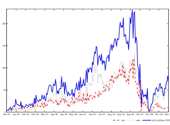
The volume of securitized assets traded in the US has grown remarkably from the beginning of the 1990s until the onset of the global financial crisis, when it collapsed. Figure 1 shows the monthly volume of issuance of asset-backed securities (ABS), mortgage-backed securities (M BS) and their sum (all) from January 1993 until De-cember 2010. Such volumes have been determinant in shaping the development of the financial markets and particularly financial intermediation, motivating several studies to analyze their effects on credit issuance and standards, focusing particularly on mortgage markets. The general message is that mortgage securitization increases loan supply and lowers aggregate price of credit. Although securitization has tra-ditionally been higher in the mortgage market, our data shows that the issuance of ABS matches the issuance of M BS in the beginning of the 2000’s. Furthermore, the participants in the market of asset-backed securities are financial entities, com-prising of financial companies and funding corporations, sometimes referred to as shadow banks, who hold a more diverse portfolio than commercial banks. As a result, due to potential portfolio effects, those high volumes of securitization might affect other asset classes. The focus of this paper, therefore, is to investigate the effects of securitization on bond and equity markets.

Figure 1: Volume of Securitization - US

Jan0−93 Jan−94 Feb−95 Feb−96 Mar−97 Apr−98 Apr−99 May−00 Jun−01 Jun−02 Jul−03 Aug−04 Aug−05 Sep−06 Oct−07 Oct−08 Nov−09 Dec−10 50

100 150 200

abs mbs all (in billion USD)

We first conduct an empirical analysis that looks at the dynamic properties of bond and equity excess returns (risk premia1) and identify the effects of variations in the volume of securitization on asset prices. The benchmark empirical specifica-tion builds upon the work of Campbell, Chan, and Viceira (2003), and sets up a general vector autoregressive (VAR) process for asset returns including the volume of securitization, the bond premium and the equity premium. Additionally, as they do, we include the short-term rate, the dividend-price ratio and the yield spread. We find that an innovation to the growth of asset-backed securitization leads to

1_{We will use excess returns and risk premia interchangeably. Note that in some studies risk}

a statistically and economically significant drop in term spreads, equity and bond premia and contributes to explain their variance. Although the benchmark empi-rical analysis focuses on the period before the crisis, we find that the relationship between securitization and asset prices seem to hold also for the post-crisis period (after 2008) and is not driven by the surge in securitization in the years preceding the crisis. We then augment the model in order to detect whether this link is re-lated to financial intermediation or whether securitization might be instrumenting for other aspects of the economy or the financial markets. As such we control for risk perceptions/aversion (vix), for the Cochrane-Piazessi factor (CP), accounting for the consumer’s heteroscedastic discount factor as suggested by Cochrane and Piazzesi (2005), for expectations about economic performance, for changes in credit conditions (credit spread) and equity payoff (expected earnings-per-share). Our re-sults remain largely unchanged and thus indicate that specific aspects of financial intermediation that are related to fluctuations in securitization affect different asset classes other than credit.

While comparing the effects of different segments of the securitization market we find that the link between securitization and asset prices is stronger with asset-backed securities than with mortgage-asset-backed securities. We believe that this is because shadow banks and security brokers and dealers became important players in the ABS market reinforcing the view that the effect occurs through the portfo-lio allocation changes due to securitization. Data from the Federal Reserve Bank Flow of Funds on total asset holdings and their growth during the 90’s and 2000’s, depicted in Figure 2, confirms the importance of these financial entities2 relative to commercial banks and other sectors in the economy (households and non-financial firms). Note that the accumulation of assets of these entities is very much linked to the volume of securitized assets issued in the US market. The growth of assets is faster during the 90’s as the volume of securitization quickly reached around 50 billion USD per month. After that, the growth rate of assets decreases during the early 2000’s while monthly volumes of issuance in the securitization markets re-mained fairly constant. Asset holdings start to increase sharply again during the next period of growth in the securitization market, from 2002/2003 until 2006/2007, when monthly issuance reached 200 billion USD. In fact, when we include both se-curitization and security broker and dealers asset holdings in our (quarterly) VAR specification we confirm this link, an innovation to the asset backed securitization leads to a sharp increase in asset holdings.

We then propose a theoretical model that can account for our empirical findings and use it to discuss the channels through which financial intermediation and par-ticularly, securitization practices, affect asset prices and risk premia. The model’s two key ingredients are: banks3 _{can create a market for securitized assets by} de-signing and selling synthetic securities (securitization decision), and select which assets to hold in their balance sheet (portfolio decision). In creating the securitiza-tion market we follow DeMarzo and Duffie (1999) closely and motivate the issuance

2_{Shadow banks comprise of financial companies, funding corporations and ABS issuers. We}

then add assets of security brokers and dealers and compare their total to that of commercial banks.

3_{Unless otherwise specified banks are generic financial entities holding a diversified portfolio of}

Figure 2: Increasing Relevance of Financial Sector

Jan0−93Jan−94Feb−95Feb−96 Mar−97 Apr−98Apr−99 May−00 Jun−01Jun−02Jul−03Aug−04 Aug−05 Sep−06Oct−07Oct−08 Nov−09 Dec−10 2000

4000 6000 8000 10000

Sec. Brokers ABS Issuers Commercial Banks Shadow Banks and Sec Brokers

(a) Financial Assets - Commercial vs Shadow Banks

Jan−930 Jan−94Feb−95Feb−96Mar−97 Apr−98Apr−99 May−00Jun−01Jun−02Jul−03Aug−04 Aug−05 Sep−06Oct−07Oct−08Nov−09 Dec−10 0.2

0.4 0.6 0.8 1 1.2 1.4 1.6 1.8

Non−financial corporates Household Commercial Banks Shadow Banks and Sec Brokers

(b) Growth of Assets in Different Sectors

of synthetic securities as a tool to create liquidity. Banks select the allocation of assets to maximize expected returns subject to two constraints: they must fund all purchases with internal and with, potentially costly, external funds and they must abide by a risk constraint. We find that securitization, or the pooling and tranching of credit assets, allows banks to expand their balance sheets since it not only relaxes the banks’ cash or funding constraint but also their risk constraint. As a result, securitization allows banks to take additional exposures not only on credit but also on bonds and equity. The desire to increase exposure in all asset classes stems from the fact that concentrating asset holdings in one class depresses returns and, due to lack of diversification, increases the shadow cost of risk. Greater asset demand increases prices and depresses risk premia, confirming the empirical results.

One of the implications of the theoretical model is that although the intrinsic characteristics of assets, their return and risk profile, have not changed, and the degree of risk aversion has remained the same, higher volumes of securitization decrease the compensation for risk bearing in the economy. In other words, there is a potential mismatch between actual and market price of risk due to the securitization process. As pointed out by Rajan (2005), reduced premia/volatility does not directly imply reduction in risk.

Related Literature

Our work is connected to three main streams of literature. Firstly, it is linked to the empirical literature that studies the effect of securitization on credit market outcomes. Loutskina and Strahan (2009) show that credit supply is sensitive to lender’s funding restrictions for illiquid loans, classified as such since they cannot be securitized, but is not sensitive to their liquid counterpart. Hence, their results indicate that high levels of securitization in the US would lead to higher loan supply. Altunbas, Gambacorta, and Marques-Ibanez (2009) look at the banking sector in Europe and conclude that securitization has strengthened banks’ capacity to supply new loans. Finally, using data from Spain, Jim´enez, Mian, Peydr´o, and Saurina (2010) conclude that wholesale finance allows banks with access to securitization to increase their credit supply and decreases the aggregate price of credit. In all cases, including ours, the common feature is that securitization leads to a balance sheet expansion of banks. However, these studies look at credit markets only, while we also consider the impact of securitization on other asset classes.

The second and main literature that our paper relates to is the one that focuses on the effect of financial intermediation on asset prices. He and Krishnamurthy (2013) show that, during periods of crisis, binding banking capital constraints help to explain the evolution of risk premia. Our results indicate that different charac-teristics of financial intermediaries’ balance sheets can be relevant in asset pricing even when banking capital is not a direct concern. Adrian, Etula, and Muir (2014) and Adrian, Moench, and Shin (2010) stress that the growth of assets in the balance sheet of security brokers and dealers influences asset prices and risk premia. These studies are the closest to ours since as the data shows securitization and balance sheet expansion of these entities are closely linked. Our added contribution is that, by looking closely at the portfolio choice of financial intermediaries and incorpo-rating one of the key aspects in their decision, namely, the ability to create and sell synthetic assets, we are able to identify the potential channels and structural parameters that link financial intermediation and asset prices. Finally, Aksoy and Basso (2014) also explore the effects of bank’s portfolio choice but focus on maturity transformation and the gap between long and short-term interest rates in a gene-ral equilibrium setting, linking financial intermediation with fluctuations in term premia.

The paper is organized as follows. Section 2 presents our empirical analysis. The theoretical model and its solution are presented in Section 3. Section 4 discusses the main implications of our results. Finally, Section 5 concludes.

2.

Empirical Analysis

Our empirical analysis focuses on establishing whether variations in the volume of securitized credit assets traded affect different asset markets, looking particularly at the dynamic patterns of risk premia in fixed income and equity markets. Our starting point is a general vector autoregression (VAR) for asset returns used by Campbell and Viceira (1999) and Campbell, Chan, and Viceira (2003). Campbell, Chan, and Viceira (2003) employ a VAR containing the returns of the main fixed income and equity assets, namely the short-term rate, the government bond excess return (bond premium) and the equity excess return (equity premium). Additio-nally, they include the dividend-price ratio and the yield/term spread (difference between short and long term rates). Given our focus on securitization we add the variation in the volume of securitized assets traded as an additional variable. Our main interest, therefore, is in assessing whether there is additional information content in fluctuations in securitization for explaining variations in excess market and bond returns and establishing the effect of a shock to this additional variable on the dynamic responses of asset returns. In order to identify these shock responses we follow the identification structure of Christiano, Eichenbaum, and Evans (1999). As such, the VAR moving average representation is given by

zt=B(L)ut, (1)

where B(L) is the matrix of moving average coefficients and z0_t = [x0_1t, $i0

t,x

0 2t]

the vector of observables. $i

t represents the securitization measure we use, with

i = {dABSt, dM BSt, dALLst} for asset backed securitization, mortgage backed

securitization and aggregate securitization, used one at a time. Note that x1t is a

(k1×1) vector with elements whose contemporaneous and lagged values influence the variables of interest at timetand x2tis a (k2×1) vector with elements whose values are only affected by an innovation to the variables of interest at time t. Finally, ut

is a (k×1) vector of reduced form errors withk =k1+ 1 +k2.We want to obtain an impact matrix A¯ linking reduced form errors (ut) to fundamental shocks (εt) such

that ut =A¯εt. We assume that A¯ has a block triangular structure with zero in its

upper diagonal.

For our benchmark analysis, we assume x1t is empty, placing all remaining

va-riables inx2t, hence the securitization variable is ordered first, being unaffected by

the other variables contemporaneously. This identification assumption reflects the fact that the securitization process normally requires the creation of a new accoun-ting entity (special purpose vehicles) that holds and commercializes the assets and the pooling and tranching of assets that are then rated by external credit agencies. As a result, it involves a time delay from decision to implementation greater than the reaction time of asset prices. Thus, it appears natural to assume that asset prices can only affect the volume of securitization with a lag.

de-velopment of the securitization market is a recent event (last 15-20 years). Moreover, given our identification and the fact that a bank’s portfolio selection should occur at much shorter frequency, we use a monthly dataset. As a result, in order to capture sufficient dynamics (particularly in fixed income return) we estimate the model with four lags. We calculate impulse responses to a securitization shock and associated one standard error bias-corrected bootstrap confidence bands as suggested by Kilian (1998). Before discussing the estimation results we present the dataset.

2.1.

Data

Our securitization data, obtained from Dealogic,4 _{consists of daily data on asset} (ABS) and mortgage backed securitization (M BS) with tranche values and deal dates completed in the US from the year 1993 onwards. Using this dataset, we are able to construct monthly time series data of the volume of transacted securities in the US financial markets. Figure 1 (depicted in the introduction) displays the levels data for both ABS and M BS securitization volumes and an aggregate measure (all), with their summation. As is clear from the figure, while securitization started from rather modest levels by early 1990s, aggregate securitization steadily increased reaching their peak in March 2007. We note that the asset backed securitization increased from a monthly average of 5.2 billion USD in 1993 to 86.4 billion USD in 2006 (a 1540% increase) and the mortgage backed securitization increased from a monthly average of 3.5 billion USD in 1993 to 93.4 billion USD in 2006 (a 2603% increase). By the second quarter of 2007 both securitization markets collapsed and volumes remained at much lower levels as compared to pre-crisis period. Figure 1 suggests that there is a structural break in the securitization process in 2007 where market of synthetic securities froze and financial institutions and/or final investors started to move away from the practice long before the full blown realization of the financial crisis in September 2008 triggered by the collapse of Lehman Brothers.5

In the VAR, we include seasonally adjusted asset and mortgage backed securi-tization transformed in monthly log differences, denoting them respectively, dABS

and dM BS.6 We also construct a monthly aggregate securitization series (alls)

being the simple sum of M BS and ABS (labeled as dALLs). Next to the securi-tization data, our empirical exercise utilizes the following data series. Benchmark monthly excess market returns (xr) annualized, obtained from the Kenneth French website, are based on Fama-French method and summarize the excess return on the (equity) market over the risk free rate (3 months T-Bill rate). We use monthly

4_{We obtain a deal report with deal type equal to ABS or MBS, currency code equal to USD,}

nationality of risk equal to USA and deal price date from beginning of 1993 until October 2014.

5_{It is clear that the actual global financial crisis started by mid 2007. As reported by the}

Investment Company Institute (2012) “in June 2007 two Bear Stearns’ hedge funds suspended redemptions in the face of deteriorating investments in securities backed by subprime mortgages. [...] In the summer and fall of 2007 a range of additional short term investment pools (both unregistered and offshore) began to fail after investing in securities backed by subprime mortgages. In February 2008 the auction rate securities market froze as securities for sale exceeded demand, auction agents refused to take the excess supply on their balance sheets, and all auctions failed.”

6_{We use Census X12 method to remove cyclical seasonal movements from securitization series}

Fama-Bliss Discount Bonds as reported by CRSP to calculate annual excess bond returns (xbr) over 2,3,4 and 5 years horizons as described in Gurkaynak, Sack, and Wright (2007) for the calculation of yields and in Cochrane and Piazzesi (2005) for the calculation of the excess bond returns, i.e. xbr_t(₊₁n) = r_t(₊₁n) −y_t(1) where xbr(_tn₊₁)

denotes thenyear excess log return,r_t(₊₁n) denotes the log holding period return from buying an n-year bond at time t and selling it as n−1 year bond at time t+ 1 and

y_t(1) denotes the log yield. We use a monthly real price dividend ratio (rpd) calcula-ted using the log difference in real dividends and real stock prices (S&P Composite Stock Price Index) as reported and updated by Robert Shiller’s stock market data. Term spreads (spread) are computed as the difference between the five year govern-ment bond rate and 3 months T-Bill in percentages per annum. Real short term rates (realr 3m) are calculated using the 3 months T-Bill rate and the CPI infla-tion. Our full sample covers the period from January 1993 up until October 2014. However, conditional mean and variances have most likely changed as a result of the financial crisis and central bank intervention, which influenced market liquidity and consequently the securitization market, preventing us from estimating the full period without accounting for the regime change. In order to do so we would need a longer post-crisis dataset than we currently have. As a result, in our benchmark VAR estimations we only use data from January 1993 till November 2007; thereby we exclude the period after the collapse of the securitization market that later on became a full blown financial crisis.7

2.2.

Estimation Results - Parsimonious model

As mentioned before our starting point is a parsimonious representation of as-set returns provided by Campbell, Chan, and Viceira (2003). We therefore as-set up the benchmark VAR withZ_t0 =$i0

t,x 0

2t

, wherex2t= [rpdt, spreadt, xbrt, xrt, realr 3mt].

Thus, the variable of interest, in a recursive fashion is log difference in securitization,

i.e. dABS ordM BS and the variables in x2t are respectively, log of dividend-price

ratio (rpd), term spreads (spread), excess bond returns over two years horizon (xbr), excess market returns (xr), and short term real rates (realr 3m).

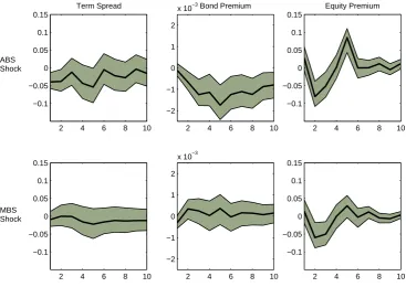
Figure 3 displays the impulse responses with respect to a shock to variations in different types of securitization. The top panels show responses to a shock in changes in ABS. We see that term spreads decline significantly. Excess bond (2Y) returns show a significant decline that lasts nearly a year. Excess equity market returns do not respond significantly instantly but suffer a sizeable and significant decline for the next quarter, rebounding quickly after that. Although we only depict the one standard deviation confidence bounds, the cumulative effect of the ABS on bond premium after 5 periods and on the equity premium after 2 periods (their respective peak effects) are both significant at 5% confidence level. The impulse responses show the effect of changes in securitization volume when all the interactions amongst the asset price variables are considered. We also run predictive return regressions8 _that

7_{Although inference is problematic due to lack of data, in one of our robustness exercises we use}

data after 2008 checking whether the link between securitization and asset prices remain unchanged, see discussion in the next section and Appendix for results.

8_{We estimate Rx}i

t+1 = αi+βi0∗Zt+εit+1, where Rxit+1 consists of excess returns on term

Figure 3: Impulse Responses - Parsimonious Model

Term Spread

2 4 6 8 10

−0.1 −0.05 0 0.05 0.1 0.15

Bond Premium

2 4 6 8 10

−2 −1 0 1 2

x 10−3 Equity Premium

2 4 6 8 10

−0.1 −0.05 0 0.05 0.1 0.15

2 4 6 8 10

−0.1 −0.05 0 0.05 0.1 0.15

2 4 6 8 10

−2 −1 0 1 2

x 10−3

2 4 6 8 10

−0.1 −0.05 0 0.05 0.1 0.15 ABS

Shock

MBS Shock

include variations in asset backed securitization among return predictors similar to Adrian, Moench, and Shin (2010). Lags of asset backed securitization negatively affect term spreads, bond and equity premia. Results show that the direct effect of the changes in securitization (its second lag) on bond and equity premium are signi-ficant at 10% and 5% confidence level, respectively (see Appendix for the regression output results).

Our results indicate that the link between the variations in the volume of secu-ritization and asset prices is not only statistically significant but also economically significant. A monthly increase of 5 billion USD in the volume of ABS9 issued in the market leads to a 6 basis point movement in bond premium after 5 periods, which implies a 10% movement in bond premium relative to its sample mean, and a 272 basis point decrease in equity premium after 2 periods, which implies a 35% movement in excess return relative to its sample mean. In order to further analyze the dynamic relationship between securitization and asset prices we also inspect the forecast error variance decompositions (FEV). We observe that by the twelfth month about 7.5% of variations in excess bond returns are attributable to shocks to varia-tions in ABS, about 20% of variations are attributable to term spread shocks and nearly 70% of variations are attributable to its own (excess bond returns) shocks. FEV analysis in the case of excess equity market returns also shows a similar

contri-vector of return predictor variables with four lags with dividend price ratio and 3-months real interest rate, lags on the excess returns next to variations in asset backed securitization. We define

Zt=rpdt, realr 3mt, dABSt, Rxit

.

9_{Apart from the period from 2004 and 2007, monthly issuance of ABS remained always bellow}

bution ofdABS. Over a twelve month horizon, approximately 46% of forecast error variance in excess market returns are attributable to shocks to dividend-price ratio, whereas 6.2% of forecast error variance of excess returns are attributable to shocks to variations in ABS. As is well known, excess market returns exhibit much less persistence, thus only 39% of its forecast error variance are attributable to its own shocks. Finally, VAR based excess market returns predictive estimation that in-cludes dABS increases its in-sample-fit (as measured by the adjusted R-squared) from 2% to 4% as compared with the VAR specification without the inclusion of

dABS.

The bottom panels exhibit responses to a shock to variations in mortgage backed securitization. We observe that, initially, spreads decline as in theABS case but the movement is statistically insignificant. Excess bond returns response to the shock is initially a decline, however it rebounds quickly and becomes insignificant. Finally excess equity market returns response to mortgage backed securitization is similar to its response to the asset backed securitization, i.e. no initial response followed by a stronger and significant decline in excess returns. Overall, we find that the response to a M BS shock is much less pronounced compared to the responses to variations in asset backed securitization. When investigating the FEV, we note that the contributions of shocks to variations inM BS to explain forecast error variance of excess bond returns is negligible and around 2% for market returns.

We also run the VAR with the aggregate measure of securitization,dALL. Given that the volume of securitization in the mortgage market (M BS) is normally greater than that of ABS, the impulse responses (not reported here) are closer to the one observed for M BS than for ABS. Overall securitization has a stronger and more significant impact on equity premium than on bond premium. The FEV for excess bond returns suggests that the role of shocks to aggregate securitization in explaining the forecast error variations in excess bond and market returns are negligible. In the case of excess market returns, the role of total securitization is more pronounced in explaining the forecast error variance. By the twelfth month about 10% of forecast error variance in excess market returns is attributable to shocks to variations in aggregate securitization. Finally, VAR based excess market returns predictive estimation that includes dALLs increases the in-sample-fit (as measured by the adjusted R-squared) from 2% to 7% as compared with the VAR specification withoutdALLs.10

We perform a series of robustness tests using the parsimonious model, focusing only on the estimation using the variation in the volume of ABS. Details are presen-ted in the appendix. Firstly, we verify whether the impact of securitization on asset prices is driven by the remarkable increase in the volume of deals during the 2003-2007 period, when many new financial instruments were introduced. We restrict the data set to the period 1993 - 2002 and find that the negative impact of inno-vations to securitization volumes on bond and equity premium remain unchanged. However, securitization shocks contribute relatively less in explaining FEV in excess bond and market returns for this sample period and the size movement in equity premium after an ABS shock is also smaller, reducing to around 150 basis point for a 5 billion monthly increase in ABS, indicating that the link between securitization

and asset prices become more relevant during the 2003-2007 period.

Secondly, we use data from January 2009 until October 2013, effectively estima-ting the period after crisis as a new regime.11 _{Although inference is impaired by the} lack of degrees of freedom, we find a similar pattern of response to both bond and equity premia, with a downward movement of bond premium, reaching its lowest level 5 periods after the securitization shock and equity premium moving down after a few periods and rebounding quickly after that. Variance decomposition analysis also paints a similar picture, with securitization shocks contributing to explaining around 6% of forecast error variance in excess bond returns and around 4.5% of FEV in excess market returns. Thus, the results indicate that the link between securitization and risk premia across other asset classes has not been substantially altered by the recent crisis, although the monthly volume of deals return to the levels observed in the early 2000’s.

Thirdly, we focus on the identification assumption by altering the ordering of the variables in the VAR. We set x2t =∅ and x1t = [rpdt, spreadt, xbrt, xrt, realr 3mt],

thus securitization can only affect asset prices with a lag, but is affected by the other variables contemporaneously. The negative effect of securitization on bond and equity premia are qualitatively unchanged. We also note that shocks to equity and bond premia12 _{do not lead to lower volume of securitization (in fact if anything} securitization tend to initially increase after these shocks), thus reverse causality does not seem to hold.

2.3.

Estimation Results - Augmented model

The results of the parsimonious model of asset return dynamics indicate there is a role for variations to the volume of asset backed securitization in explaining the fluctuations in excess bond and excess market returns. Mortgage backed securitiza-tion does not appear to be linked to excess bond returns, although it has significant effects on the equity premium (thus variation in the total volume of securitization explains a significant part of variations in excess market returns). In order to in-crease our understanding of the added value of looking at the securitization markets to explain risk premia, and assess the robustness of our results, we augment the benchmark model in several directions, particularly focusing on the potential effects of omitted variables.

We subdivide the vector x2t = [x2at,x2bt], such thatx2bt = [rpdt, spreadt, xbrt,

xrt, realr 3mt] contains all the variables included into the benchmark model and

x2at represents additional controls. That way, all controls, together with the

securi-tization can have a contemporaneous effect on asset returns. We now explain each control and the rationale for including them.

It is possible that including measures of securitization may be serving as instru-ments for changes in some aggregate risk perception criteria. In order to try and correct for possible biases due to this omission, we incorporate a market volatility

11_{Note that we need one year ahead data to calculate bond premia.}

12_{In order to analyze the effect of, for instance, a shock of bond premium, we set x}

1t = xbrt

and the remaining variables as part ofx2t, thus bond premium can affect securitization

measure and setx2at =vixt. The CBOE Volatility Index (vix) captures the investor

sentiment and market volatility embedded in the near-term volatility conveyed by S&P 500 market index option prices as provided by Bloomberg.

Securitization may also be related to future economic performance, as perceived by market participants. In order to account for that we include a measure of consu-mer expectation about future economic conditions: E5Y index is derived from a five years forward looking question on confidence from the Michigan Index of Consumer Expectations (see Barsky and Sims (2011) and Aksoy and Basso (2014) for different applications of the relation between E5Y and future economic activity).

Of course, securitization practices may not be directly linked to general econo-mic performance but could be linked to positive news on firm performance that in-crease credit and equity payoffs. Thus, we firstly incorporate the expected earnings-per-share (deps), which is calculated by using the twelve months forward weighted average expected earnings per share based on S&P 500 composite as reported by I/B/E/S. Secondly, we include a control for aggregate credit spread level using the credit spread index proposed by Gilchrist and Zakrajsek (2012), settingx2at =GZt.

Finally, Cochrane and Piazzesi (2005) have shown that the five year government bond forward rate is a useful predictor of the excess returns on two year bonds when we abandon the expectations hypothesis. Their explanation is based on the consumption Euler condition. When bond prices are determined by the expected re-lative marginal utilities divided by inflation, a conditionally heteroscedastic discount factor will generate time varying bond risk premium. Therefore, if financial inter-mediaries securitization decision is unrelated to the consumption Euler condition, we should see additional information content in variations in securitization next to Cochrane-Piazessi factor (CP); so we set alternatively x2at =CPt.

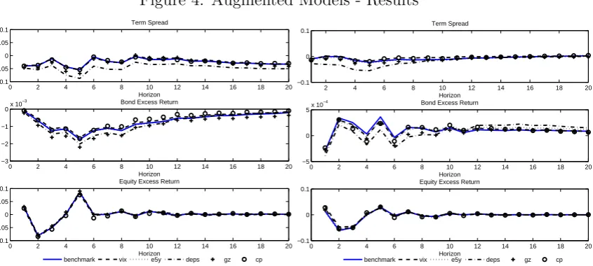
Figure 4 displays the corresponding impulse responses that include one of the additional controls at a time whendABS and when dM BS are used as the securi-tization measure, respectively. An inspection of those figures suggests that impulse responses remain broadly the same after the inclusion of different controls. Hence, we conclude that a shock to changes in asset backed securitization leads to a decline in term premium, equity and bond premia, while there is no significant impact of a shock to mortgage backed securitization on excess bond returns and a negative but a relatively smaller effect on excess returns on equity.

Figure 4: Augmented Models - Results

0 2 4 6 8 10 12 14 16 18 20

−0.1 −0.05 0 0.05 0.1

Horizon Term Spread

benchmark vix e5y deps gz cp

0 2 4 6 8 10 12 14 16 18 20

−3 −2 −1

0x 10

−3

Horizon Bond Excess Return

0 2 4 6 8 10 12 14 16 18 20

−0.1 −0.05 0 0.05 0.1

Horizon Equity Excess Return

(a) Impulse Response to Asset-backed Securities

2 4 6 8 10 12 14 16 18 20

−0.1 0 0.1

Horizon Term Spread

benchmark vix e5y deps gz cp

0 2 4 6 8 10 12 14 16 18 20

−5 0 5x 10

−4

Horizon Bond Excess Return

0 2 4 6 8 10 12 14 16 18 20

−0.1 0 0.1

Horizon Equity Excess Return

(b) Impulse Response to Mortgage-backed Securi-ties

controlling for it does not affect the shape of the impulse responses nor the FEV contribution of ABS shocks. By the twelfth month, the shocks to dABS account for about 6% of FEV decompositions in bond excess returns while the CP factor account for nearly 71% of variations.

The empirical results, therefore, indicate that securitization impacts negatively, both, the bond and the equity premia. Moreover, this explanatory power is not related to the potential link between the changes in the volume of transactions in the securitization market with the degree of risk perception/aversion of agents, intertemporal consumption Euler conditions, or with the general economic or credit and equity returns outlook. As a result, the channel through which this effect occurs may be more directly related to the functioning of financial intermediation when the originate to distribute mode of operation is more heavily employed. Given that our results are stronger when the volume of asset-backed securities is used instead of the one of mortgage backed securities, one must look at shadow banks and security brokers and dealers, which are more active in that niche of the market relative to traditional commercial banks. Furthermore, shadow banks and brokers and dealers normally hold a more diverse portfolio of assets that are not only concentrated on credit products but also contain equity and fixed income products, making the potential portfolio effects of the high activity in securitization markets more likely to be observed.

variables included in the estimation. Results are presented in the Appendix. From the first estimation we observe that a securitization shock leads to lower equity pre-mia and term spreads, although the effect on bond premium is insignificant. When security brokers and dealers assets are included, the effect of securitization on risk premia are quantitatively the same and as expected we also observe that asset hol-dings respond positively to a securitization shock. Finally, when securitization is excluded we find that the impact of innovations to the growth rate of asset holdings does not lead to significant changes to risk premia. We believe both our results and theirs are complementary, pointing to the importance of financial intermediation in explaining asset prices. By focusing on the volume of securitization, we highlight the potential mechanism through which this link occurs. Consequently, in order to increase our understanding of the potential channels through which securitization and financial intermediation activity affects asset prices we build a model of finan-cial intermediation where securitization is used as a form of funding by a finanfinan-cial entity (bank) who holds a diverse portfolio of assets that include credit, government bonds and equity. We turn to that next.

3.

Model

In order to provide a rationale for the empirical results presented above, we build a partial equilibrium model that focuses particularly on the portfolio choice of banks when securitization of credit assets held on the balance sheet is feasible. As such, banks will face two key decisions: the securitization decision, which entails the creation of the securitization market by designing and selling synthetic securities, and the portfolio decision of which assets to hold on their balance sheet.

Initially, there are three assets available for the bank to invest in, credit assets (loans), denoted Yi for i ∈ [1, n], government bonds (B), and equity (E). Banks

will select a portfolio of assets to maximize expected returns (profit) facing two constraints: (i) a cash constraint, as asset purchases must be funded by internal funds (capital) and external funds, which comprise of direct bank borrowing and po-tential resources prevenient from the securitization market and (ii) a risk constraint, such that banks care about risk.

A fourth asset, denoted F, will be created by the bank. We assume the bank creates a Special Purpose Vehicle (henceforth, SPV) which will serve as the agent commercializing this asset to final investors. Banks are willing to securitize assets since they have a preference for liquidity13 (denoted byδ), which is passed on to the SPV. This assumption ensures securitization is a cheaper form of funding relative to direct borrowing. The payoff ofF will be a function of the performance of the basket of credit assets [Yi]ni=1, depending on the security design. We assume banks receive information about the payoff structure of credit assets [Yi]ni=1 that is not available to the market at large, hence, the key component influencing the securitization market will be the existence of this information asymmetry.

13_{Liquidity generation is not the only reason for securitizing assets. This may occur due to}

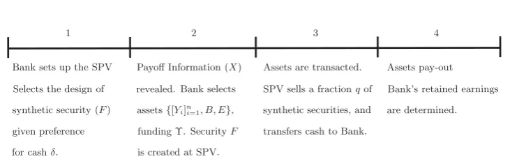
In order to simplify the exposition and its solution, we divide the model into four stages. In the first stage the bank sets up the SPV, selecting the design of security

F. During stage 2 the bank receives private information not available to the market at large and selects its portfolio composition. At stage 3 all assets are transacted and in the final stage uncertainty is revealed and assets pay-out. Figure 5 shows the timeline of the model.

Figure 5: Model Timeline

Bank sets up the SPV

Selects the design of

synthetic security (F)

given preference

for cashδ.

Payoff Information (X)

revealed. Bank selects

assets{[Yi]ni=1, B, E},

funding Υ. SecurityF

is created at SPV.

Assets are transacted.

SPV sells a fractionqof

synthetic securities, and

transfers cash to Bank.

Assets pay-out

Bank’s retained earnings

are determined.

1 2 3 4

3.1.

Securitization Decision

The securitization decision involves the design of the synthetic security and the setting up of the SPV. Based on that the equilibrium in the securitization market is obtained, allowing the quantity of asset F that is transacted and the price to be determined. These variables will then be used in the portfolio decision to be explained next. Hence, the key assumption is that the securitization and portfolio decisions can be solved independently. This is accomplished by assuming that the SPV only cares about the liquidity generated from the securitization market and that the equilibrium in this market is independent from the portfolio allocation (we relax the second assumption in section 3.4). The securitization part of the model follows DeMarzo and Duffie (1999) and DeMarzo (2005) closely. In order to determine the security design and the market equilibrium we introduce a number of assumptions regarding the credit assets.

Each assetihas a final payoff ofYi =Xi+Zi. The componentXi represents the

bank’s private information about the payoff of the credit asset that is not available to other investors. Zi represents the remaining risk the bank faces. We assume Zi

can be divided into two components, an idiosyncratic part and an aggregate credit market component, thusZi =i+η. LetYn≡Pn_i=1Yidenote the cumulative payoff

of credit assets and Y ≡(Y1, . . . , Yn) the vector of assets. Same definitions hold for

X,Xn, Z, and Zn. Finally, let X−i ≡(X1, . . . , Xi−1, Xi+1, . . . , Xn).

We then make the following assumptions

• A1. E[Zi |X] = 0 orE[Yi |X] =Xi.

• A2. Given anyX−i, the conditional support ofXi is a closed interval and has

greatest lower boundXi0 >0.

Assumptions 1 and 2 guarantee thatX comprises all information available onY, that given the information on all other assets, there is still a range of possible infor-mation states for asset i, and that the lower bound of that range is independent of

X−i. Finally, Assumption 3 ensures enough regularity on the distribution of shocks

to allow for the determination of the security design.

The securitization market and the creation of SPV

We assume the bank issues synthetic securitiesF and place them on the balance sheet of an SPV. The key characteristic of the SPV is its preference for transforming these securities in cash, or a liquidity preference. We denote this preference by parameter δ.14 _{Based on that, the SPV selects the amount q of synthetic securities} to sell. LetPF(q) denote the price of the synthetic security F whenq units are sold,

or the demand schedule for security F. Then the SPV selects q equals to

arg max

q∈[0,1]qPF(q) +δ(1−q)E[F |X] = arg maxq∈[0,1]q(PF(q)−δE[F |X]) (2)

Thus, the preference for liquidity implies that assets not sold are discounted relative to the cash gains from transacted synthetic securities. Therefore, the key characteristic of the SPV is its desire to sell as much securities F as possible, since it prefers holding cash (and transferring it back to the bank) than holding F on its balance sheet (although its price might be equal to its expected value). The main obstacle for the SPV or for the functioning of the securitization market is the existence of information asymmetries between the final investor and the SPV. Given its preference for liquidity, if the securityF is priced according to its value based on all information available, let that price be f =E[F |X], then the SPV would want to publicly offer all stock of synthetic securities or set q = 1. Would final investors be willing to buy all the stock of synthetic securities? Final investors do not have the same information set as the bank and will be trying to determine the appropriate price. Assume he/she bids the lowest possible price (linked to the lower bound of

X, denoted f0 = E[F | X = X0]). On the on hand, if the SPV/bank receives a signal X > X0, the value of the security is higher than the price bid by the final investor and thus the SPV may not be willing to sell all the stock of securities F, offering only a lower proportion to the market (q <1), thus indicating to investors that the security is better than expected and its price should be greater than f0. On the other hand, if the SPV received the worst possible signal (X =X0), it will sell all securities confirming the final investor’s initial expectation. Hence, given a bid price of PF, the public offer of the SPV (q) will convey information about the

bank’s private information on the conditional payoff of the security. In summary, the SPV security retention (offering q < 1) is a credible signal (of higher X) since retention is costly due to its preference for liquidity. The market equilibrium (PF, q)

is thus the equilibrium of a signalling game in which uninformed investors compete for purchases of the security being offered by the SPV in a Walrasian market setting. DeMarzo and Duffie (1999) provide the following characterization of this equili-brium.

Under assumptions A1 - A2,

q = (f /f0)−1/(1−δ) and PF =f0(q)δ−1 =f (3)

is a unique separating equilibrium. The SPV payoff function will be ΠSP V_{(f, f}

0) =

q(PF(q)−δE[F | X]) = f0(1−δ)(f /f0)−δ/(1−δ), where f = E[F | X], and f0 =

E[F |X =X0]. The equilibrium is obtained by solving (2), conditional on PF =f,

and imposing the boundary condition that PF(1) =f0.

Optimal Design of F

Having obtained the characterization of the equilibrium in the securitization market we can now solve backwards to determine the security design (stage 1 in the model15_{). Given the timeline of the model the synthetic security design is done} before X is revealed to the bank. Hence, the optimal design problem is given by maxF(.)E[ΠSP V(f, f0)]. DeMarzo and Duffie (1999) and DeMarzo (2005) show that under assumptionsA1 - A3 the optimal monotone security design is a standard debt contract.16 That isF∗(Y) = min(d, Yn) for a constant d(face value). The intuition is simple. The bank/SPV would like to maximize the volume of securitized assets, but due to the information asymmetry, is forced to retain some synthetic assets in the portfolio when the signal is good and information asymmetry is high. Hence, it is optimal for the SPV to select a security that is as payoff insensitive as possible for the range of signals where asymmetry is at its highest. Standard debt has this property since f does not change significantly as X increases in the range X d. That way, the bank problem is

max

d E[Π SP V

(fd, f₀d)], where fd=E[min(d, Yn)|X].

In order to provide further characterization on the debt contract, PF and q,

we assume that η ∼ N(0, σ2_{) (recall that η is the aggregate credit shock affecting} all credit assets) and Xn is uniformly distributed between X0 =

P

ixi0 and X1 =

P

ixi1. As we increase the number of securities n, the value of f becomes

f_nd = E[min(d, Xn+ (1/n)Xi+η)|X]→E[min(d, Xn+η)|X] =fd

fd =

Z (d−Xn)

−∞

(Xn+η)f(η)dη+

Z ∞

(d−Xn₎

df(η)dη

where f(η) is the density function of η

fd = XnΦ

d−Xn

σ

+d

1−Φ

d−Xn

σ

−σφ

d−Xn

σ

where Φ(·) and φ(·) are the standard normal cumulative and density functions

15_{Note that we do not need to determine the decision in stage 2 since the optimal design and}

the portfolio decision are independent.

16_{We are assuming the bank will find it optimal to pool all credit assets together and set a debt}

contract dependent onYn, instead of issuing a securityF for each asset Yi. As DeMarzo (2005)

shows, for a large number of securities in the pool, when the variance of the idiosyncratic risk i

Also note thatfd

0 =X0Φ d−_σX0

+d 1−Φ d−X0

σ

−σφ d−X0

σ

. The aggregate shockη, which is not diversified away as the basket of credit is constructed can also be understood as the correlation risk amongst assets Yi, for i ∈ [1, n], within the

basket.

Based on the solution for fd and f₀d, d∗ is given by

d∗ = arg max

Z X1

X0

(1−δ)(f₀d)1/(1−δ)(fd)−δ/(1−δ) 1 (X1−X0)

dX (4)

We are not able to obtain an analytical solution to this integral and thus offer a description of the main trade-off involved in the selection of the optimal face value,

d∗. Due to the presence of information asymmetry the SPV is forced to retain a fraction (1−q) of synthetic securities. That is costly since it prevents the SPV from maximizing liquidity creation. Hence, one of the drivers behind the selection of d∗

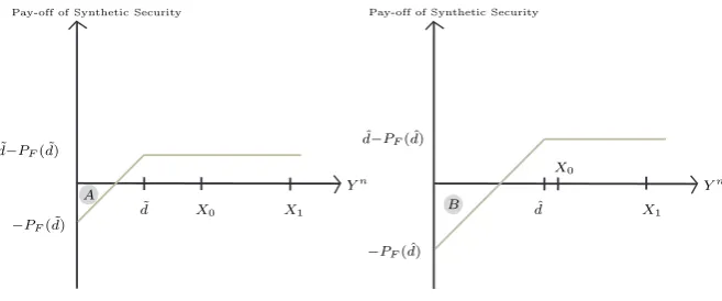
is to minimize the information sensitivity of F. Figure 6 shows the pay-off of the synthetic security to the final investor for a low value of d= ˜d (left-hand side) and for a high value of d = ˆd < X0, also depicting the range of possible information

Xn_∈[X

0, X1]. On the one hand, when dis small, the probability thatYn (payoff of credit) is such that the payoff of final investors is negative (regionA) is quite small (far away from range [X0, X1]) and the actual loss is also small. On the other hand, whendis high the probability that Yn_{is such that the payoff is negative (regionB)}

is greater (not far from range [X0, X1]) and the potential loss more sizeable. Hence, ford= ˆdit is relevant from the point of view of the final investor to know ifXn_=X

0 orXn _=X

1, while when d= ˜d it is not as much. That is, the bank wants to select

d∗ as small as possible to minimize the information sensitivity of F, maximizing q. However, as the bank decreasesd∗, it also decreasesPF(d∗) since d∗ > PF(d∗). As a

result, total cash for each unit of synthetic security sold is smaller. Thus, the desire to maximize cash receipts from securitization through the price of security pushes

d∗ up. Optimal d∗ balances the trade-off between these two effects, maximizing

PF(d∗)q(d∗).

Figure 6: Synthetic Security Payoff and Optimal d

X0

X0 X1 dˆ X1

˜

d

Yn

Yn

ˆ

d−PF( ˆd)

˜

d−PF( ˜d)

−PF( ˆd) A

B

Pay-off of Synthetic Security Pay-off of Synthetic Security

−PF( ˜d)

3.2.

Portfolio decision

Banks select a portfolio of equity, government bonds and credit to maximize expected returns. Banks invest in three main assets: credit assets (loans), denoted

Yi for i ∈ [1, n], government bonds (B), and equity (E). Given the assumptions

made on the returns of credit assets [Yi]ni=1, and the fact that banks pool all these assets to design the synthetic security, instead of looking at each asset i, we can concentrate directly on the credit basket whose payoff is equal toYn_{. Let Q}

y be the

quantity of pooled credit assets the banks buy. Recall that due to the diversification of idiosyncratic risks (i), the only source of risk of the basket of credit comes from

the aggregate uncertainty (η). We assume the price of the basket is given by its expected payoff conditional on the banks information set Py = E[Yn | Xn], but

also that the bank can extract a credit mark-up (denoted µ(Xn_{, Q}

y)) while acting

as a financial intermediary. Although we do not model that explicitly this could be due to the its informational advantage as in DeMarzo (2005), or because it has some bargaining power over firms/agents that make loans. We assume µ(Xn_{, Q}

y) is

a function of (i) the signal Xn_{; the greater X}n _{relative to the lower bound X}

0 the greater the bank’s information advantage and thus higher the mark-up; and (ii) the quantity transacted Qy; the greater the bank’s demand for credit assets (supply of

loans), the lower its mark-up. Thus, for µ1, µ2 >0, we assume

µ(Xn, Qy) = ¯µ+µ1(Xn−X0)/X0−µ2Qy. (5)

Government bonds payoff is given by VB. We assume VB ∼ N($B, σ2B). Banks

buy QB units of bonds and pay price PB for each unit. Equity payoff is given by

VE. We assume VE ∼ N($E, σ2E). Banks buy QE units of equity and pay a unit

price PE. Banks take prices PE and PB as given while selecting their portfolio

composition. Prices are then determined in equilibrium based on market demand schedules PB(QB) and PE(QE) given by

PB =αB+βBQB (6)

PE =αE +βEQE. (7)

In order to fund these assets, banks utilize internal funds (capital), denoted by Γ0, and external funds. These consist of direct bank borrowing (Υ) and resources prevenient from the securitization market, which, from the results in the previous section, comprise of qPF for each unit of pooled credit asset (Qy). As a result

of the separation between the securitization and portfolio decisions, the bank, at this stage, takes (q, PF, f, f0,) as given. The cost of bank borrowing is given by

RF = ¯R+κ(Υ/Γ0). Thus, we assume the cost of external funding increases from a base rate ¯R as borrowing increases relative to the amount of bank capital. Bank profits/returns (ΠB) are then given by

ΠB|Xn = Qy(Yn−Py) +µ(Xn, Qy)Qy

+QB(VB−PB) +QE(VE −PE)−qQy(F −PF)−RFΥ. (8)

We assume banks select the portfolio composition (Qy, QB, QE,Υ) to maximize

the expected profits E[ΠB | Xn] subject to two constraints. The first asserts that the cost of purchase of assets is equal to the amount of funds, or a cash constraint. That is given by

The second ensures the bank abides by a limit on risk taking or a risk constraint.17 It is common to assume that this constraint takes the form of the first percentile of the distribution of expected returns, or a Value-at-risk constraint. Although widely used in practice this type of constraint introduces complexity to the portfolio problem. Instead, we assume that the bank faces a limit to the standard deviation of the portfolio returns. If the assets in the portfolio were only credit, bonds and equity, given the assumption on normally distributed payoff, the two constraints (limit on standard deviation and on the percentile of the distribution) are equivalent. When synthetic products are incorporated the two may diverge since assetF’s payoff distribution is not symmetric.

The standard deviation of the portfolio returns is given by

σ_ΠB |Xn = Q2_yσ2+Q2_Bσ_B2 +Q2_Eσ_E2 + 2Q_yQ_Bσ_yB+ 2Q_yQ_Eσ_yE+

2QBQEσEB−2qQ2yσF Y −2qQyQBσF B −2qQyQEσF E+q2Q2yσF2 1/2

.

Whereσabis the covariance between the payoff of securitiesaandb, andσF2 is the

variance of the synthetic security. The risk constraint limits the standard deviation of the bank profits to be smaller or equal to a fraction of the total capital of the bank. This fraction (χ), denotes the degree of risk aversion of the bank. Thus, the portfolio choice must be such that

σ_ΠB 6χΓ₀. (10)

Given the security design and the solution for fd we can now determine the variance and covariances that involve the synthetic security F. These are (details can be found in the Appendix)

σ2

F|Xn = (Xn)2Φ(d

−Xn

σ )−2Xnσφ( d−Xn

σ )−σ2[ d−Xn

σ φ( d−Xn

σ )−Φ( d−Xn

σ )]+d2[1−Φ( d−Xn

σ )]−(fd)2

σF y|Xn = (Xn)2Φ(d−_σXn)−2Xnσφ(d−_σXn)

−σ2[d−_σXnφ(d−_σXn)−Φ(d−_σXn)]+d[Xn(1−Φ(d−_σXn))+σφ(d−_σXn)]−fdXn

σF B|Xn ≈ Φ(d−_σXn)σyB

σF E|Xn ≈ Φ(d−σXn)σyE

The portfolio problem is given by

max {Qy,QB,QE,Υ}

E[ΠB |Xn] s.t. (9) and (10) (11)

Note that as a solution to this problem is obtained, one can find the shadow value (in term of profits) of an extra unit of cash holding to the bank (Lagrange multiplier of the cash constraint, denoted λc). We can use this multiplier to pin

down the value of δ, the bank’s liquidity preference, or the discount factor of the SPV. Essentially, we will set δ = 1−λc, where λc is obtained when the portfolio

decision is solved while settingq = 0, or without securitization. This way we assess the bank’s desire to obtain cash from securitization.

3.3.

Model Results

The equilibrium of the model is defined as the vector of asset allocations {Qy,

QB,QE, Υ,q} and the vector of prices{µ, PB, PE, PF, d} such that (i) given prices,

{Qy, QB, QE,Υ} solves problem (11); (ii) {q, PF} is a separating equilibrium of

the signalling game; (iii) the face value of debt d is given by (4); and (iv) given {Qy, QB, QE}, prices {µ, PB, PE} are consistent with the credit spread (mark-up),

(5), and the market demand schedules (6) and (7).

Our main interest is to verify the effect of securitization on the portfolio allocation of banks, and through that, its effect on asset risk premia. The bond risk premia in our model can be defined as BP(QB) ≡ E[VB]−PB, while the equity risk premia

is given by EP(QE) ≡ E[VE] −PE. Given that the portfolio decisions and the

equilibrium in the securitization market are a function of the information setXn _∈

[X0, X1], the equilibrium is obtained for Xn within that interval. Note that when

Xn _{= X}

0, banks do not have an information advantage over the market, since the existence of the lower bound X0 is known. However, as Xn increases from

X0, banks have an advantage in determining the true value of the credit basket, hence, the degree of information asymmetry between final investors and the bank increases. We solve the model for two cases, one where we constrain q = 0, hence the market of securitization is disregarded (denotedModel No Sec) and one whereq, the securitization volume, is obtained based on the separating equilibrium described above (denoted Model with Sec).

Due to the non-linearity of the risk constraint and the integral needed to be solved to obtain the face value of debt (see (4)) we can only obtain numerical solutions. The parameters used in the benchmark specification are shown in Table 1.18 _Starting from the return parameters, we set the mean payoff on bonds to be around 5% and the mean payoff on equity to be that plus 3%. The parameters {αB, αE} are set

such that if banks do not buy any bonds or equity the risk premia on each asset are slightly above their mean average in the data used in the empirical section. Parameters {βB, βE} control the sensitivity of the risk premia to increases in bank

asset demand. This is set such that if the bank uses all its capital to buy one asset it offsets most of the premia, ensuring bank portfolios are not concentrated in one asset. We set the credit basket to pay a mark-up slightly greater than the equity premium since credit is the riskier asset. The variance and covariance structure is based on the data for government bond returns, the return on the S&P500 and the credit spread index (GZ) proposed by Gilchrist and Zakrajsek (2012). Using this data we find that the standard deviation of equity returns is 60% the standard deviation of credit spreads, while that ratio is 20% for the case of government bonds. All asset payoffs are found to be negatively correlated as reported in the table. We set X0 to be equal to 1.02 and the degree of information asymmetry m, given by the different between X0 and X1, is set to 0.2 (two times the standard deviation of the aggregate shock). Finally, we set δ to be equal to 1 minus the Lagrange multiplier obtained from the solution of the bank portfolio when securitization is not performed and limit the standard deviation of the portfolio to be 7% of the banking capital (under normally distributed returns that would imply limiting the

18_{Although no calibration exercise is done we attempt to select parameters based on the relevant}

loss under the first percentile (Value-at-risk) to roughly 25% of bank capital). We perform different sensitivity analysis to most of the parameters described in table 1 to verify the robustness of our predictions, but also as a tool to increase the understanding of the key mechanism behind the impact of securitization on risk premia.

Table 1: Parameter Values - Benchmark Model

Return Variance Bank

$E 0.03+1/0.95 σY 0.1 δ 0.983

$B 1/0.95 σB 0.02 Γ0 5

αB $B - 0.02 σE 0.06 χ 0.07

αE $B +0.01 ρEY -0.49

βB _Γ1₀0.025 ρEB -0.57

βE _Γ1₀0.025 ρBY -0.4

¯

R 0.01

κ _Γ1

00.05 Information

µ1 0.01 X0 1.02

µ2 _Γ1₀0.005 m 0.2

¯

µ 0.04 X1 X0 +m

3.3.1. Benchmark model

We start by presenting the results of the benchmark model. Figure 7 shows the difference between the equilibrium of the full model (M odel with Sec) and the one obtained by settingq = 0, or restricting the bank to do no securitization. We report the bond and equity premia, the final credit market spread or mark-up (µ(Xn_{, Q}

y)),

the bank’s asset holdings/balance sheet (Qy+QB+QE), the amount of securitization

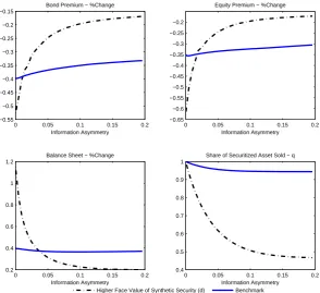
(q) and finally the percentage point change in the ratio of external borrowing and bank capital, measuring the degree of leverage based on direct borrowing. The results are shown for the entire range Xn ∈ [X0, X1].19 Note that the degree of information asymmetry in the market is directly related to the difference betweenXn

and the lower boundX0, which is known. Hence, we define information asymmetry as the ratio (Xn−X0)/X0.

Firstly, allowing for securitization to be conducted implies the bank is able to increase its asset holdings (balance sheet) across all the range of information asym-metries ([0,(X1−X0)/X0]). This increase pushes bond premium, equity premium and credit mark-up down. Second, securitization is at its highest when information asymmetry is at its lowest. The SPV does not need to retain any synthetic security when it does not have an informational advantage relative to final investors. As in-formation asymmetry increases it must retain a greater portion of synthetic assets, not being able to exploit the securitization market as much. As a result, balance sheet expansion generally decreases with more information asymmetry,20and conse-quently, the equilibrium bond and equity premium respond less. The balance sheet

19_{We smooth the final solution to correct for potential inaccuracies in the numerical optimization}

solution, see the Appendix for more details.

20_{The increase observed as X}n _{→ X}

Figure 7: Benchmark Model

0 0.05 0.1 0.15 0.2 −40 −39 −38 −37 −36 −35 −34 −33

Bond Premium − %Change

Information Asymmetry

0 0.05 0.1 0.15 0.2 −36 −35 −34 −33 −32 −31 −30

Equity Premium − %Change

Information Asymmetry

Effect of Allowing Banks to Securitize Credit Assets (Model with Sec vs Model No Sec)

0 0.05 0.1 0.15 0.2 −1.4 −1.3 −1.2 −1.1 −1 −0.9 −0.8 −0.7

Credit Spread − %Change

Information Asymmetry

0 0.05 0.1 0.15 0.2 0.94 0.95 0.96 0.97 0.98 0.99 1

Share of Securitized Asset Sold − q

Information Asymmetry

0 0.05 0.1 0.15 0.2 36 36.5 37 37.5 38 38.5 39 39.5 40

Balance Sheet − %Change

Information Asymmetry

0 0.05 0.1 0.15 0.2 −19

−18.5 −18 −17.5 −17

External Borrowing/Γ₀ − %PointChange

Information Asymmetry

expansion affects all three assets for two main reasons: (i) due to market demand sensitivity concentrating all expansion in one asset reduces the return on that asset relative to the others, and (ii) due to diversification gains banks are able to manage risk exposures more effectively by increasing allocation of all assets. Another inter-esting feature is the effect of securitization on the liabilities side of the balance sheet. We observe that securitization replaces external borrowing as a source of funding, in fact securitization becomes the main source of funding. Leverage based on external borrowing (Υ) decreases significantly relative to the case when securitization is not allowed.

Hence, the key conclusion of the theoretical model is that although the intrinsic characteristics of the assets (payoff and risk) in the banks portfolio has not changed and the bank’s degree of risk aversion (represented by parameter χ) has remained the same, we observe that the risk premia required to maintain those assets on the balance sheet decrease substantially as securitization is employed. This confirms the empirical results presented in section 2. We find that an increase in securitization implies a drop in risk premia after controlling for a set of variables that are related to the future payoff of the assets (e.g. dividend/price ratios, earnings-per-share, consu-mer expectations) or the degree of risk aversion in the market (e. g. vix). The main driver of the volume of securitization is the degree of information asymmetry. Thus, through the portfolio selection of the bank, the degree of information asymmetry in credit markets leads to variation in risk premia.

credit assets are becoming relatively better assets andPF increases withXn and thus the liquidity

This portfolio channel is present due to the effect of securitization on the two main constraints the bank faces. Firstly, while external funds are costly since direct borrowing must carry an interest rate that is increasing as bank leverage increases, banks are able to acquire funds by creating and selling the synthetic securities that are linked to their balance sheet holdings at significantly lower costs. Thus, securi-tization relaxes the bank’s cash constraint. Secondly, by designing a debt contract as the format of the synthetic security the bank is also decreasing the extent of risk taking in credit markets. To see this compare the payoff of a (naked) credit basket (left panel in Figure 8), the short position on the synthetic security (middle panel in Figure 8) and a portfolio that combines a long position on the basket and a short position on the synthetic security (or the final portfolio of the bank after securitization, depicted in the right panel of Figure 8). The short position on the synthetic security essentially protects the bank against losses when the credit bas-ket payoff (Yn) is lower than the face value of debt (d). Thus, securitization also relaxes the bank’s risk constraint.21 _{As a result, banks find it optimal to increase} asset holdings. Since banks have a preference for diversification both due to the risk constraint and the negative expected gain from overbidding in one single market, banks increase holding of all asset classes. Therefore, securitization of credit implies low risk premia across all asset classes.

Figure 8: Risk Profile

Pay-off Credit

−Xn

Xn

Yn

Yn

Yn

Pay-out Synthetic Sec. (F)

PF

(PF−d)

d d

Combined Portfolio Pay-off

(PF−Xn)

In the benchmark model we assume banks select d optimally to maximize the SPV gains from securitization. Given that the key aim is to decrease the effects of information asymmetry and thus reduce SPV retention of synthetic securities, banks set d∗ quite low (optimal d is 0.81, significantly lower than X0 = 1.02).22 As a result, the proportion of securitized assets traded (q) is greater than 0.94 for all Xn. However d∗ also has implications for the degree of risk protection a short position on synthetic securities provide. This protection increases with d. We thus solve the securitization equilibrium and the portfolio decision when d = 1.15×d∗, or the face value is 15% greater than in the benchmark case.23 This change has

21_{Note that securitization affects the left tail of the distribution of returns and thus the fact we}

use a constraint on the standard deviation instead of a constraint on the first percentile of losses decreases the risk protection provided by securitization. This would be stronger for a standard Value-at-Risk constraint, increasing the effects of securitization on risk premia.

22_{Settingdlow is effectively the same as attempting to create AAA (safe) tranches, whose price}

will then be insensitive to asymmetric information. Increasing d, for the same underlying asset, generates lower rated tranches or riskier synthetic securities.

23_{That implies in this alternative equilibrium definition only (i), (ii) and (iv) are satisfied (see}