International Journal of Emerging Technology and Advanced Engineering
Website: www.ijetae.com (ISSN 2250-2459, Volume 2, Issue 8, August 2012)212
Design and Analysis of Pole-Placement Controller for
Interconnected Power Systems
Naimul Hasan
Department of Electrical Engineering Jamia Millia Islamia, New Delhi-110025, India Abstract - Pole placement is a control method assigned to
arbitrary closed loop poles by state or output feedback. In linear systems, poles have influence on stability, system response, and transient response of the system. The applications of pole placement technique in power system operation and control have been found a significant place over the years. This paper presents salient features of pole placement technique in the design of controllers in power systems. Following this, as an application the AGC regulators are designed for a two area interconnected power system and their feasibility is tested by implementing these regulators in the wake of 1% load disturbance in one of the areas. The dynamic performance achieved with the designed AGC regulators is compared with that obtained with optimal AGC regulator designs based on full state vector feedback control concept. The investigations of the results achieved demonstrate the superiority of AGC regulators designed using pole placement technique over the optimal AGC regulators in all aspects of system dynamic response characteristics.
Keywords - AGC, AC link, Load frequency control, Pole placement, linear time-invariant system
I. INTRODUCTION
For a successful operation of a power system, the system parameters like, frequency, voltage profile, reliability, security etc. must be maintained at their nominal values throughout its operation. The system is kept to operate between the various system operating limits as prescribed by system constrains. As the electrical power system is always associated with continuous changes in operating conditions, the operational and control aspects require dedicated means and tools to deal such changing operating conditions and make the overall power system operation as successful.
The structure of present day power systems is very huge and complex. Furthermore, the sharing of benefits in utilizing the variability in generation mixes and load patterns with other technological reasons, most of the power systems are put to operate in electrically interconnected manner evolving in to a vast structured power grids which are subdivided into regional operating groups called power pools or power areas. ]
The operation of power system as an interconnected system usually leads to improved system security and economy of operation [1]. In addition, the interconnection permits the utilities to make economy transfers and thus take the advantage of the most economical sources of power. The benefits have been recognized from the beginning and interconnections continue to grow. However, the operation and control of such systems becomes more difficult.
One of the most important control aspects of interconnected power systems is to keep system frequency at scheduled level under the varying load and generation condition. The system frequency has been varying with changing load conditions. With primary speed control action, a change in system load will result in a steady-state frequency deviation, depending upon the governor droop characteristic and frequency sensitivity of the load. All generating units on speed governing will contribute to the overall change in generation, irrespective of the location of the load change. Restoration of system frequency to nominal value requires supplementary control action which adjusts the load reference set point. As system load is continually changing, it is necessary to change the output of generators automatically [2].
The primary objectives of automatic generation control (AGC) are to regulate frequency to the specified nominal value and to maintain the interchange power between control areas at the scheduled values by adjusting the output of selected generators [2,3].
International Journal of Emerging Technology and Advanced Engineering
Website: www.ijetae.com (ISSN 2250-2459, Volume 2, Issue 8, August 2012)The present article deals with an AGC regulator design for an interconnected power system model. The designed AGC regulators are implemented in the wake of load disturbance in one of the two areas. The system dynamic performance obtained with (i) AGC regulator designed using pole placement technique and (ii) AGC regulator designed using full state vector feedback control concept under the same system operating conditions.
II.
DESIGN OF OPTIMAL AGCREGULATORThe state space representation of a linear time invariant system can be given by the following differential equations;
d/dt[x(t)]=Ax(t)+Bu(t)+Ed(t) (1) y(t)= C x(t (2)
To design an optimal regulator for the system described by equations (1) & (2), one has to find a control law of the form;
u = - K x (3)
which minimizes the performance index (J*) given as;
J* = 1/2
0 [xTQ x+uTRu] dt (4)
Where Q and R satisfy the definiteness conditions Q ≥ 0 and R > 0.
To Determine the optimal feedback matrix „K‟, which minimizes the performance index, is the standard optimal regulator design problem. The matrix „K‟ is obtained by solving the following matrix Riccati equation.
S+ATS+SA-SBR-1BTS+Q=0 (5)
It can be shown, that the value of „K‟ that minimizes the J* is given by;
K= R-1BTS (6)
The acceptable solution of „K‟ is that for which the system remains stable. The system dynamics with feedback is defined by;
dx/dt = (A – B K)x (7)
Moreover, for stability of the closed loop system, all the eigenvalues of the matrix (A – B K) should have negative real parts.
III. POLE-PLACEMENT TECHNIQUE
In certain applications, a preselected degree of damping is required and, at the same time, the optimization of the control effort is essential [12-14].
In these cases it is necessary to achieve predetermined closed-loop eigenvalues and simultaneously minimize a
cost function. In general, it is not possible to minimize an arbitrary quadratic performance index and, at the same time, achieve predetermined closed-loop eigenvalues. Some techniques, however, have been developed that achieve the desired closed-loop eigenvalues and simultaneously compute suitable weighting matrices in order to optimize the quadratic performance index. The problem of optimal pole-placement has been generally solved only in the case of single-input linear systems [13]. For the case of multi-input systems a method deals with system eigenvalues as a whole and locates them either to the left of a line Re(s)=-a in the complex plane with a selected a>0, or in a specified region of minimum damping ratio [14].
IV. POWER SYSTEM MODEL UNDER INVESTIGATION
A 2-area interconnected power system consisting of identical thermal power plant with reheat turbines is selected for the investigation. The optimal AGC regulators are designed using the pole placement technique. The transfer function model of the system under consideration is shown in Fig.12.
V. DEVELOPMENT OF SYSTEM STATE SPACE MODEL
The following differential equations are achieved from the transfer function model of Fig.1.
In the transfer function model, the parameters M1 and D1 are defined as:
M1= Tp1 / Kp1 = f
H1
2
D1= 1/Kp1
d/dt(F1)=(Pg1-Ptie-Pd1)(1/M1)-(D1/M1)F1 (8)
d/dt(Pr1)=Xg1 (Kt1/Tt1) -PR1/Tt1 (9)
d/dt(Pg1)= -Pg1/Tr1+Pr1(1/Tr1-Kr1/Tt1)+Xg1(Kr1
Kt1/Tt1) (10)
d/dt(Xg1)=Pc1(Kg1/Tg1)-F1(Kg1/R1Tg1)- Xg1/Tg1
(11) Similarly the following differential equations can be derived
d/dt(F2)=(Pg2-a12 Ptie-Pd2) (1/M2) -(D2/M2)F2
(12)
d/dt(PR2)=Xg2(Kt2/Tt2)-PR2/Tt2 (13)
d/dt(Pg2) = -Pg2/Tr2+PR2(1/Tr2-Kr2/Tt2)+Xg2
(Kr2Kt2/Tt2) (14)
d/dt(Xg2) = Pc2 (Kg2/Tg2) -F2 (Kg2/ R2Tg2) -
International Journal of Emerging Technology and Advanced Engineering
Website: www.ijetae.com (ISSN 2250-2459, Volume 2, Issue 8, August 2012)Considering the linearized model of incremental tie-line power flow, the expression for total incremental tie-line power exported from area „i‟ can be written as:
Ptiei =
s
p 1
2Tip(Fi dt-Fp dt) (16)
where „p‟ represents the number of control areas. The differential equation for incremental tie-line power flowing from area 1 to 2 can be written as:
d/dt(Ptie)=T(F1-F2) (17)
The integrals of area control errors of both areas IACE1 and IACE2 are derived as follows:
IACE1=(Ptie1+B1F1)dt (18)
IACE2=(Ptie2 +B2F2)dt (19)
State, control and disturbance vectors
With the help of equations (1) & (2) and differential equations (8)-(19), the structure of matrices A, B and Fd can be derived.
State Vector
[X]T=[ΔF1 ΔPg1 Δ Pr1 ΔXg1 ΔF2 ΔPg2 ΔPr2 ΔXg2 ΔPtie
∫ACE1 ∫ACE2]
Control Vector
U =
2 1
C C P
P
Disturbance Vector
Pd = 2 1
d d
P P
State Matrix A
[(-1/Tp1)(Kp1/Tp1)0 0 0 0 0 0(-Kp1/Tp1)0 0 0-1/Tr1 1/Tr1-(Kr1/Tt1 Kt1Kr1/Tt1 0 0 0 0 0 0 0 0 0 (-1/Tt1) (Kt1/Tt1) 0 0 0 0 0 0 0
(-Kg1/(R1*Tg1)) 0 0 (-1/Tg1) 0 0 0 0 0 0 0 0 0 0 0 -1/Tp2(Kp2/Tp2) 0 0 ((-a12*Kp2)/Tp2) 0 0 0 0 0 0 0 -1/Tr2 1/Tr2-Kr2/Tt2 Kt2*Kr2/Tt2 0 0 0 0 0 0 0 0 0 (-1/Tt2) (Kt2/Tt2) 0 0 0
0 0 0 0 ((-Kg2)/(R2*Tg2)) 0 0 (-1/Tg2) 0 0 0 (2*pi*T12) 0 0 0 (-2*pi*T12) 0 0 0 1 0 0 b1 0 0 0 0 0 0 0 1 0 0
0 0 0 0 b2 0 0 0 -1 0 0]
Control Matrix B
BT=[0 0;0 0;0 0;Kg1/Tg1 0;0 Kg2/Tg2;
0 0;0 0;0 0;0 0;0 0;0 0;]
Disturbance Matrix Fd
FdT=[-Kp1/Tp1 0;0 0; 0 0;0 0;0 -Kp2/Tp2
;0 0;0 0;0 0; 0 0;0 0; 0 0;]
Coefficient matrices
The system coefficient matrices A, B, E, C, for the power system model can be determined with the help of numerical values of power system parameters involved in the structure of these matrices and the compensated system
matrix AF based on the pole placement is determined by
(A-B*K)
State Cost Weighting Matrix ‘Q’
The matrix „Q‟ is selected as an identity matrix of the order 11x11.
Control Cost Weighting Matrix ‘R’
The control cost-weighting matrix „R‟ is a 2x2 dimensional identity matrix
VI. SIMULATION RESULTS
For the simulation study, MATLAB-7.0 software is used. The feedback gains of optimal AGC regulators are obtained for power system model under consideration. These gains are shown in Table-1and Table-2 respectively. The closed loop system eigenvalues are computed to investigate the system dynamic stability with the implementation of designed AGC regulators. The pattern of closed-loop system eigenvalues are given in Table-3. And the performance indices is shown for both regulators in Table-4. The system dynamic response plots are plotted with the implementation of optimal AGC regulators using full state feed and pole placement technique in the wake of 1% load disturbance in either of the two areas. The response plots obtained are shown in Figs. (1-11).
Table-1 Optimal Feedback Gains
[0.3834 3.2563 0.8552 0.2463 0.1959 0.0190 -0.0749 0.1205 -0.5731 0.7431 -0.4870
0.5065 2.3298 0.3283 0.3099 1.6553 0.2717 -0.0558 -0.0514 -2.0516 1.0855 0.6342]
Table-2
International Journal of Emerging Technology and Advanced Engineering
Website: www.ijetae.com (ISSN 2250-2459, Volume 2, Issue 8, August 2012)[
0.3182 1.060 -0.1388 0.4155 -0.0449 -0.02530.0263 -0.0137 -0.1133 0.5068 -0.1910 0.047 0.1037 0.0335 0.0449 0.3746 0.0177 -0.0235 -0.0549 -0.6144 -0.0047 0.4519]
Table-3
Closed-loop System Eigenvalues
without Pole Placed With Pole Placed
-20.1312 -13.6534± 2.4331i -2.6262 ± 4.5277i -4.3404 -3.5953 -0.3443 ± 0.1599i -0.3748
-0.1977
-24.2353 -17.0544± 0.4278i
-2.5863± 4.3883i
-4.7158 -3.6243
-0.3762 ± 0.1445i
-0.3676 -0.1979
Table-4 Performance Index
without Pole Placed With Pole Placed
28.1861
22.1647
VII. DISCUSSION OF RESULTS
Table 1 and 2 list the optimal feedback gain matrices for the model under consideration. From the inspection of feedback gains obtained for both the case study, it is observed that there is an appreciable reduction in the values of feedback gains of optimal AGC regulators designed with pole placement technique as compared to that obtained with full state vector feedback control strategy. The closed-loop system stability is ensured for both optimal AGC regulators based on the full state feedback and pole placement techniques.
The investigation of the time response plots of frequency deviation in area-1and area-2 as shown in Figs. 1 and 5 reveal that there is a reduction on in the magnitude of first peak of responses achieved with implementation of optimal AGC regulators designed using pole placement technique as compared to that obtained with optimal AGC regulators designed using full state vector feedback control strategy.
The other positive aspect of output pole placement strategy is with the reduction of oscillatory modes around steady state value in these time responses. The similar trends are also visible in the response plots.
VIII. CONCLUSIONS
From the investigations of results, it is revealed that there is an appreciable reduction in the magnitude of first peak of responses with proposed optimal AGC regulator designed using the pole placement technique as compared to that obtained without the pole placed at teir optimal position. And other this positive aspect of pole place placement technique is with the reduction of oscillatory modes, smooth and the settling time of system responses around steady state value are fast as compared to in these time responses.
Numerical data [2].
REFERENCES
[1 ] N. Cohn, “Considerations in the regulation of interconnected area,” IEEE Trans., Power Systems, PAS-86, pp. 1527-1538, Dec. 1967. [2 ] P. Kundur, Power System Stability and Control. New York:
McGraw- Hill, 1994.
[3 ] O. I. Elgerd and C. Fosha, “Optimum megawatt frequency control of multi-area electric energy systems,” IEEE Trans. Power Apparatus System, vol. PAS-89, no. 4, pp. 556–563, Apr. 1970.
[4 ] J. E. Van Ness, “Root loci of load frequency control systems,” IEEE Trans., Power Apparatus and Systems, PAS (82), pp. 712-726, 1963. [5 ] Ibraheem, Prabhat Kumar, and Dwarka P. Kothari, “Recent philosophies of automatic generation control strategies in power systems”, IEEE Trans. Power Syst., vol. 11, no. 3, pp. 346-357, February 2005.
[6 ] W. R. Barcelo, “Effect of power plant response on optimum load frequency control system design,” IEEE Trans., Power Apparatus and Systems, PAS(92), pp. 254-258, 1973.
[7 ] C. E. Fosha & O. I. Elgerd, “The megawatt frequency control problem: A new approach via optimal control theory,” IEEE Trans on Power Apparatus and Systems, PAS-89 (4), pp. 563-577, April 1970.
[8 ] M. Athans and P. L. Falb. Optimal Control. New York: McGraw-Hill, 1966.
[9 ] A.T.Alexandridis and G.D.Galanos, “Optimal pole placement for linear multi input controllable system”, IEEE transaction on Circuit and System, vol. CAS-34, no. 12, pp. 1602-1604 December 1987. [10 ]W. M. Wonham, “On pole-assignment in multi-input controllable
linear systems.” IEEE Truns. Automat. Contr., vol. AC-12, pp. 660-665, 1967.
[11 ]M. Athans, “The role and use of the stochastic lag problem in control system design,” IEEE Transc. Automut. Contr., vol. AC-16, pp. 529-552, 1971.
[12 ]B. Porter and J. J. D‟Azzo, “Closed-loop eigen structure assignment by state feedback in multivariable linear systems,” Jnt. J. Contr., vol. 27, pp. 487-492, 1978.
[13 ]B. P. Molinari, “The state regulator problem and its inverse,” IEEE Trans. Automat. Contr., vol. AC-18, pp. 454-459, Oct. 1973. [14 ]B. D. 0. Anderson and J. B. Moore, “Linear system
International Journal of Emerging Technology and Advanced Engineering
Website: www.ijetae.com (ISSN 2250-2459, Volume 2, Issue 8, August 2012)0 5 10 15 20 25 30 35 40 -1.4
-1.2 -1 -0.8 -0.6 -0.4 -0.2 0 0.2
D
E
L
F
1
Time (sec)
Without poleplacement with Pole Placement
Fig 1. Response of F1 for 1% load disturbance in area-1
Time (sec)
0 5 10 15 20 25 30 35 40
0 0.2 0.4 0.6 0.8 1 1.2 1.4
D
E
L
P
g
2
without pole placement with pole placement
Fig 2. Response of Pg1 for 1% load disturbance in area-1
0 5 10 15 20 25 30 35 40
0 0.2 0.4 0.6 0.8 1 1.2 1.4
D
E
L
P
r1
Time (sec)
without pole placement with pole placement
Fig 3. Response of Pr1 for 1% load disturbance in area-1
0 5 10 15 20 25 30 35 40
0 0.2 0.4 0.6 0.8 1 1.2 1.4
D
E
L
X
g
1
Time (sec)
without pole placement with pole placement
Fig 4. Response of Xg1 for 1% load disturbance in area-1
0 5 10 15 20 25 30 35 40 -1.4
-1.2 -1 -0.8 -0.6 -0.4 -0.2 0 0.2
D
E
L
F
2
Time (sec)
Without poleplacement with Pole Placement
Fig 5. Response of F1 for 1% load disturbance in area-2
0 5 10 15 20 25 30 35 40
-0.05 0 0.05 0.1 0.15 0.2 0.25 0.3
D
E
L
P
g
2
Time (sec)
without pole placement with pole placement
International Journal of Emerging Technology and Advanced Engineering
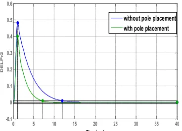
Website: www.ijetae.com (ISSN 2250-2459, Volume 2, Issue 8, August 2012)Fig 7. Response of Pr2 for 1% load disturbance in area-1
0 5 10 15 20 25 30 35 40 -0.1
0 0.1 0.2 0.3 0.4 0.5 0.6
D
E
L
X
g
2
Time (sec)
without pole placement with pole placement
Fig 8. Response of Xg2 for 1% load disturbance in area-1
0 5 10 15 20 25 30 35 40 -1.2
-1 -0.8 -0.6 -0.4 -0.2 0 0.2
D
E
L
P
t
ie
Time (sec)
without poleplacement with pole placement
Fig 9. Response of Ptie for 1% load disturbance in area-1
0 5 10 15 20 25 30 35 40
-4 -3.5 -3 -2.5 -2 -1.5 -1 -0.5 0
IA
C
E
1
Time (sec)
without pole placement with pole placement
Fig 10. Response of IACE1 for 1% load disturbance in area-1
0 5 10 15 20 25 30 35 40 0
0.5 1 1.5
IA
C
E
2
Time (sec)
without pole placement with pole placement
[image:6.612.354.533.151.279.2]Fig 11. Response of IACE2 for 1% load disturbance in area-1
1 / R1
Pc1 (1+sKr1)
(1+sTr1)
Kg1
( 1+sTg1)
Kt1
( 1+sTt1)
Pg2
T12 / s
1 / R2
(1+sKr2)
(1+sTr2)
Kp2
( +sTp2)
Kg2
( 1+sTg2)
Kt2
( 1+sTt2)
Ptie
+
+
a12
Xg2 PR2
_
_ +
_
Pc2
B1
1/s
B2
ACE1 dt
1/s +
Xg1 PR1 Pg1 Kp1
(1+sTp1) Pd1
- -
Pd2 F2
- + _
ACE2 dt
+
F1
a12
ACE1 = B1F1+Ptie
Ptie1
ACE2 = B2F2+Ptie
Ptie2
+ +
+ +
Fig 12. transfer function model of two-area interconnected power system consisting of reheat turbines
0 5 10 15 20 25 30 35 40
-0.1 0 0.1 0.2 0.3 0.4 0.5 0.6
D
E
L
P
r2
Time (sec)
[image:6.612.76.260.313.443.2] [image:6.612.324.518.468.622.2] [image:6.612.79.258.471.594.2]