Design and Modeling of State Feedback with Integral Controller for a Non-linear Spherical tank Process

(1)

International Journal of Emerging Technology and Advanced Engineering

Website: www.ijetae.com (ISSN 2250-2459, Volume 2, Issue 11, November 2012)

668

Design and Modeling of State Feedback with Integral

Controller for a Non-linear Spherical tank Process

1

D.Pradeepkannan,

2

Dr.S.Sathiyamoorthy

1

Asst.Prof/EIE, K.L.N College of Engineering, Tamil Nadu, India 2_{Professor/EIE, J.J. College of Engineering and Technology, Tiruchirrappalli}

Abstract— This paper presents the design and modeling of State Feedback with integral controller to implement in a Non-linear Spherical Tank SISO process. By using state feedback, it controls the liquid level in the tank as desired .The aim of this paper is to compare the control performance between State feedback with integral controller with conventional ZN, Luyben Tyreus PI/PID, Controllers. The mathematical model of the system is derived and verified. The simulations are carried out in MATLAB environment and their performances are compared in terms of settling time , peak time and peak overshoot.

Keywords— Integral control,State feedback control, Non linear spherical tank process.

I. INTRODUCTION

The control of liquid level is a basic problem in Process Industries such as Petrochemical industries, Paper making processes, Mixing process in a chemical plant, Water treatment plants, Chemical recovery of Fertilizer industry etc. It is essential for control system engineers to understand the working of tank control system and how the level control problems are solved. The problem of level control in a nonlinear tank process with variable area is very cumbersome. In designing the control structures Many control methods such as Adaptive Control Systems[1], Auto tuning PID [2], Ziegler- Nichols tuning [3] Full state feedback with and without Integral control [4],[5], where pole placement design via Bass and Gura‟s approach [6]is proposed. The full state feedback controller via pole placement is chosen since it has the best performance compared to other controllers in terms of oscillations and settling time[7].

Moreover, the pole placement design could also handle systems with time varying state space representation, Hence it has been applied to non linear spherical tank processes for solving their problems.

The paper is organized as follows. The section I give a brief introduction of the project The section II brief about the mathematical modeling of the non-linear spherical tank process. In section III the concepts of state feedback with integral control technique are presented and subsequently in Section IV implementation of state feedback with integral control technique for the spherical tank process.

The simulated results for ZN PI, PID, Luyben & Tyreus PI, PID are compared with state feedback with integral control given in section V. Finally, conclusion is given in section VI.

II.MATHEMATICAL MODELLING

Fig:1 Schematic diagram of Spherical Tank process A spherical time system, shown in figure 1 is essentially a system with non linear dynamics. The spherical time system has a maximum height of 1.5 metre, maximum radius of 0.7 metre. The level of the tank at any instant is determined by using the mass balance equation given below: let,

q1(t) – inlet flow rate to the tank in m 3

/sec q2(t) – outlet flow rate of the tank in m3/sec H- height of the spherical tank in meter. r – radius of tank in meter(0.75 meter).

xo – thickness of pipe in meter(0.06 meter). inlet water flow from the pump

q t

₁

( )

.Using law of conservation of mass the non-linear plant equation is obtained.

For the spherical tank,

1

1 2 1

dh

q (t) q (t)

A(h )

dt





₍₁₎

Where, 2

surface

(2)

International Journal of Emerging Technology and Advanced Engineering

669

Fig:2 Radius of the surface of the level

Radius on the surface of the fluid varies according to the level (height) of fluid in the tank. Thus let this radius be known as

r

_surface.

2

1 1

2

surface

r  rhh

2

s s

A (2rh h ) (2) And

2 0

q (t) a 2g(h x ) where,

a (x 2)

 

 

(3)

Solving (2) and (3) in eqn (1) for linearizing the non linearity in spherical tank gives rise to a transfer function of

2

1 s s

s o

a 2gH(s)

Q (s) (2rh h )SH(s)

2 h x

   



Rearranging,

2 s s

s 0

H(s) 1

Q(s) a 2g

(2rh h )S

2 h x



  



(4)

Applying the steady state conditions values the linearized plant transfer function is given by ,

( ) 0.5897 ( ) 0.004

Y S

U S S (5) 2.1 Black box modeling

Consider the first order system with dead time [8] represented by the following transfer function

( )

1

d

t s p

p

k e

G s

s









(6)

The output response to a step change in input is given by,



( ) _p (1 exp( ( ) / _p))

y t  k u   t   for t> (7) The measured output is in deviation variable form. The three process parameters

K

_p

,

 

_p

,

can be estimated by performing a single step test on process input.

The process gain is found as simply the long term change in process output to the change in process input. The time delay is the amount of time, after the input change, before a significant output response is observed. There are several ways to estimate time constant for this model. Two point method is used for estimating the process as shown in figure (5). The process gain is calculated by

changeinprocessOutput Kp

changeinprocessInput 

  

System identification for spherical tank system is done by using black box modeling in MatLAB environment. Using the open loop method, for given change in input variable the output response for system is recorded. Ziegler-Nichols have obtained the time constant and time delay of a first order plus dead time (FOPDT)[10] Model by constructing the tangent to the experimental open loop step response at its point of instruction. The tangent intersects with the time axis at the step origin provides a time delay estimate, the time constant estimated by calculating the tangent intersection to the steady state output value divided by the model gain.

( )

,

1

d

t s p

p p

k e

y

G s

k

s

u













and the values of

146.62,

1 y

u

 

2.2 Estimation of time constant by two point method Smith has obtained the parameters of FOPDT transverse function model by letting the response of actual system and that of the model to meet the two points which describe that parameter



_p

&

t

_d. Here, time required for the process output to make 28.3% and 63.2% respectively are measured. The time constant and time delay can be estimated from the equation given below,

(2 / 3) ( / 3) , 0.7

/ 3 0.4 4.644 p

d p

t t

t t 



 

  

And the values of 2

146.62, 1, 379.28 , 142.14

3 3

t t

y u s s

     

On substituting the values we obtain the FOPDT model as

k_p146.62,_p237.14s

4.644 146.62 ( )

237.14 1

s e G s

s  

(3)

International Journal of Emerging Technology and Advanced Engineering

670

The parameters of the controllers as per Ziegler Nichols tuning method are found as follows,

180 _tan 1 ₁₈₀

co dt co p

  

 

    

Substituting the values of



_p&

t

_d we obtain the value

of _co as 0.34rad/sec and _u 2 co

P 



 =18.48 and

k

_cu is

found to be 0.55.

For a ZN- PI and ZN-PID controller, the values of controller parameters are determined as

1

0.45 , 0.2475, 15.4 , 0.0161 1.2

u

c cu c i i

P

k  k k     s k  s

1

0.6 , 0.33, 9.24 , 0.0357 2

2.31 , 0.7623 . 8

u

c cu c i i

u

d d

P

k k k s k s

P

s k s





     

  

Similarly the controller parameters for Luyben and Tyreus are determined by using the formula tabulated Below in table1.

Parameter PI controller

PID controller

kc Kcu/3.2 Kcu/3.2

i 2.2Pu 2.2Pu

d Kcu/2.2 Pu/6.3

For a Luyben Tyreus- PI and PID controller, the values of controller parameters are determined as

1

/ 3.2,

0.1718,

2.2 40.66 ,

0.004

c cu c i i

k



k







Pu



s k



s



1 / 3.2, 0.25, 2.2 40.66 , 0.0062

2.93 , 0.7325 . 6.3

c cu c i i

u

d d

k k k Pu s k s

P

s k s





    

  

III. STATE FEEDBACK WITH INTEGRAL CONTROL CONCEPT

The concept of feed backing all the state variables back to the input of the system through a suitable feedback matrix in the control strategy is known as state variable feedback control technique as shown in fig. 3. Using this approach ,the closed loop Eigen values of the system will be specified. Thus the aim is to design a feedback controller that will move some or all of the open loop poles of the measured system to the desired closed loop pole locations as specified. Hence this approach is also known as pole placement control design.

The block diagram in Fig3 shows the structure of a state feedback with integral control system that composed of plant, controller and the controller parameters block.

Fig3: Block diagram of state feedback with integral control system One way to introduce integral control is to augment the state vector with the desired integral. More specifically, we can feedback the state x as well as the integral of the error in output by augmenting the plant state x with the extra „integral state‟ z , defined by the equation,

Where r is the constant reference input of the system. Since z t( ) satisfies the differential equation

0

( ) ( ( ) ) (6)

t

z t 



y t r dt  

.

( ) ( )  ( )

z t y t r cx t r (7)

It is easily included by augmenting the original system .

( ) ( ) ( ) ( ) ( )

x t Ax t bu t

y t cx t

 



as follows

.

x A 0 x b 0

u r

c 0 z 0 1

z

         

  _ _{    } _{ }

  _ _{    } _{ }

 

(8)

Since r is constant , in the steady state .

x

=0 , .

z

=0, provided that the system is stable .This means that the steady-state solutions

x z

_s_, _sand

u

_smust satisfy the equation,

s

s s

x

0 A 0 b

r u

z

c 0 0

1

  _ __{ } _{ }

   _ __{ }_{ }

  _ __{ } _{ }

  

Substituting this for the last term in equation (8) gives

.

s

s .

s

x x

x A 0 b

(u u ) (9) z z

c 0 0

z

  _ __ _ _ _{ }

  _ __ __{ }    

  _ __  _ _{ }

 

(4)

International Journal of Emerging Technology and Advanced Engineering

671

~ ~

s

s s

x

; u

(u

u )

z z









_

_









(10)

In terms of these variables , equation (9) becomes



A x bu



~ _A ₀ _b

x , b

c 0 0

   

_ _ _{ }

   

The significance of this result is that , by defining the deviations from steady-state as state and control variables the design problem has been reformulated to be the standard regulator problem , with

x

=0 as the desired state . We assume that an asymptotically stable solution to this problem exists , and is given by,

u

 

k x

Partitioning k appropriately and using and using equation (5) yields,

p i k[k k ]

s p i

uu [k k ] s p s i s s

x x

k (x x ) k (z z ) z z

  

      _ 

 

The steady-state terms must balance , therefore

0

( ( ) ) (11) t

p i p i

u k x k z  k x k



y t r dt

The control, thus , consists of proportional state feedback and integral control of output error. At steady-state ,

~

0;

x



therefore , .

lim ( )

tz t

0 or lim ( )

ty t

 r

Thus , by integrating action , the output y is driven to the no-offset condition.

This will be true even in the presence of constant

disturbances acting on the plant. Block diagram of the Fig 4: shows the configuration of feedback control system

with proportional state feedback and integral control of output error.

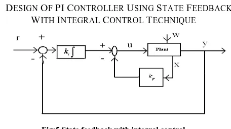
[image:4.612.332.560.133.261.2]

IV. DESIGN OF PI CONTROLLER USING STATE FEEDBACK WITH INTEGRAL CONTROL TECHNIQUE

Fig:5 State feedback with integral control The closed loop transfer function is

( ) 0.5897

( ) 0.004

Y S U S S

( ) 0.004 ( ) 0.5897 ( ) sy s  y s  u s

.

0.004 0.5897

y y u

Assigning, the state variables , we get

The completely controllable SISO linear time-invariant system with nth-order state variable model

.

x A 0 x b

u

c 0 z 0

z

          _ _{    }          

.

x 0.004 0 x 0.5897

u

1 0 z 0

z

  __ _{   } _   _ _{   } _          

The characteristic equation is

1

2 k 0.5897 (SI A)

k 0

 

 _ __{ }    =0 2

1 2

(0.004 0.5897 ) 0.5897 0

s   k s k 

The desired characteristic poles for 2

0.707, n 0.0014

  

The desired characteristic pole equation is given by , s22_ns_n2=0

(5)

International Journal of Emerging Technology and Advanced Engineering

672

Equating the coefficients of eqn (7) & (8)

1 p 0.1288 k k 

2 i 0.0054

k  k

The simulations are carried out in matlab2009A environment and the performances measure such as % peak overshoot and settling time is tabulated below in tab.2 with their controller parameters.

Parameter ZN Tuning Luyben & Tyreus

State feed back

PI PID PI PID

Kp 0.2475 0.33 0.1718 0.25 0.1288

Ki 0.0161 0.0357 0.004 0.006 0.0054

Kd - 0.7623 - 0.732 -

% peak over shoot

17.49 25 9.9 11.19 4.1513

Settling time

51.1 63.03 129 123 10.76

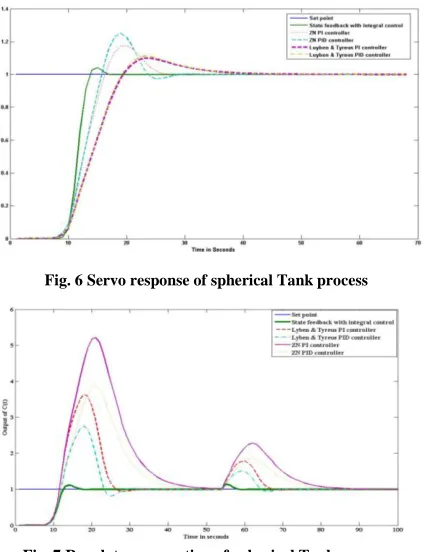
V. SIMULATION RESULTS

[image:5.612.46.291.234.377.2]

The simulated result for servo operation and regulatory operation are shown in Fig:6 .&7

Fig. 6 Servo response of spherical Tank process

VI.CONCLUSION

It has been shown that State feedback with integral controller can cope with the tank non-linear characteristics at all operating points. Conversely, Ziegler Nichols tuning method based PI controller/PID controllers and Luyben Tyreus PI/PID controllers are not able to settle at predefined time period without overshoots as desired. Hence the response of state feedback with integral control can provide better results

as tabulated with lesser settling time and with minimal overshoot.

REFERENCES

[1 ] Boonsrimuang P., Numsomran A and Kangwanrat S. " Design of PI Controller using MRAC Techniques for couple-tanks Process, World academic science engineering and Technology. Page no. (67- 72), Vol.59, 2009

[2 ] Astrom K.J., and T.Hagglund(1995).”PID controllers :Theory , design and Tuning “, Instrument Society of America ,second edition. [3 ] B.Wayne Bequette. (2003) Process control, Modelling, Design ,

and simulation, PHI

[4 ] M.Gopal. " Digital control and state variable methods conventional and intelligent control systems, Third edition.

[5 ] N.S.Nice ,.‟Control System Engineering „, John Wiley &sons.,4th

Edition. page no (764-767)2004.

[6 ] P.N.Paraskevopoulos, Digital Control System,Printice Hall. page no (156-157)1996.

[7 ] G.Sub.,D.S.Hyun,J.Park,K.D.Lee,S.G.Lee,”Design of a Poleplacement controller for reducing Oscillationsand settling time in a two inertia motor system”.27th _{Annual Conference of the IEEE}

Industrial Electronics Society.2001.

[8 ] J.H.Chow.”A Pole Placement Design approach for systems with multiple operating conditions.”IEEE transactions of Automatic control.1990.

[9 ] G. Sakthivel, T.S. Anandhi and S.P. Natarajan, Design of Fuzzy Logic Controller for a Spherical tank system and its Real time implementation.IJERA,Vol 1 Issue 3, PP 934

[10 ]S.Nithya,T.Balasubramanian,N.Sivakumaran, N.Anantharaman ,Model based controller design for a spherical tank process in real time.,IJSSST,vol-9,Nov-2008,pp(25-31).

[image:5.612.65.278.410.686.2]