Analysis of Clustering Algorithms for Data Management in Sensor Cloud

(1)

Page 270

Analysis of Clustering Algorithms for Data Management in

Sensor-Cloud

Anjali J Rathod

1

_{, Daneshwari I Hatti}

2

1

_{PG Scholar, Dept. of ECE, BLDEA’s Engineering College, Vijayapur, Karnataka, India}

2

_{Assistant Professor, Dept. of ECE, BLDEA’s Engineering College, Vijayapur, Karnataka, India}

---*---Abstract -**

In this work, ‘Data management’ and

‘Information retrieval’ in the Sensor Cloud is done by applying the Data preprocessing and Mining techniques. The enormous data in the Sensor cloud is compressed by using compression techniques such as ‘Burrows-wheeler transform’ and ‘Move-to-front coding’. Then clustering algorithms such as ‘Hierarchical and K-means algorithm’ is applied. Performance measures of these algorithms are verified by using ‘Silhouette and ‘Davies-Bouldin index’. The simulation is done in ‘MATLAB R2010a’ tool by comparing the clustering techniques.

Key Words:

Clustering algorithms, Davies-Bouldin

index, Data compression, Sensor cloud, Silhouette

index.

1. INTRODUCTION

Wireless Sensor Networks (WSNs) is a combination of several sensor equipped devices that are interconnected spatially through the wireless media, which is used to sense, collect and monitor the requirements or situations of different areas like environment such as temperature and internal functions of human body [1,2]. Each sensor device has a processing unit, storage facility, converters like Analog to digital converters (ADC), energy suppliers like batteries and transceiver[3].

Because of the several advantages of WSNs like capacity to cover broad regions, to handle the moving devices and has resistant power to deal with the node failures by taking some other path. Applications of WSNs are increasing in various fields such as healthcare, environmental monitoring and so forth.

But WSNs have limitations such as lower transmission rate, battery driven, limited energy supply, limited storage and processing capabilities [3]. Due to these limitations, it is difficult to store and process the huge amount of sensor data, which reduces the quality of data and performance of the network.

To overcome these limitations, “CLOUD COMPUTING” is an efficient technology which is called as the future

generation model. According to the US National Institute of Standards and Technology (NIST) [1], “It is defined as model for providing the automatic access to the resources such as memory, services and applications with the minimum efforts of service providers.

To solve the problem of limited power computation and limited storage capacity of the sensor network, it is necessary to integrate the sensor network with the cloud, as it provides vast storage and processing capabilities. Therefore, this integration results in the cloud computing model called “SENSOR CLOUD”.

According to the Micro Strain’s [1], Sensor cloud is defined as “It is the only storage device for the sensor data and distant management platform that is used to control the several effective cloud computing technologies which results in user analysis form”. With the help of gateway, Sensor Cloud collects the enormous amount of data from the several sensor nodes, as it provides vast storage of the data. Then, this gathered information is processed and stored in the cloud, so that other users with different applications can share the data.

As the sensor cloud collects plenty of information from several sensors, more memory is required to store the data and more energy is consumed to handle the data. Hence, it is difficult to handle and store the huge amount of data for long period of time as it consumes more amount of memory and energy and it takes more time to retrieve the relevant information(information retrieval) needed by the user from the sensor cloud.

“DATA COMPRESSION” and “DATA CLUSTERING” are the Data Preprocessing and Data Mining techniques from which data management, storage of the data, energy saving and information retrieval can be done in an efficient manner.

Data compression is a method of reducing the size of the original data set by using the transformation or encoding mechanism, such as ‘Burrows-Wheeler transform’ and ‘Move-to-Front coding’ [4].

(2)

Page 271

the data, in such a way that data in the same group (called

cluster) are more similar to each other to those in the other groups [5, 6].

2. LITERATURE SURVEY

In [1] presents the limitations of WSN such as limited storage and processing capabilities, security and privacy. To overcome these limitations cloud is integrated with WSN, which results in Sensor-Cloud. A brief overview of Sensor-Cloud architecture, advantages, applications and issues of Sensor-Cloud are discussed.

In [2] problems of WSN in terms of design and resource constraints are discussed, which is solved by integrating the WSN with the cloud and three areas are discussed namely: Sensor cloud database, Cloud based sensor data processing and sensor data sharing platform, where integration of WSN and cloud is carried out. Comparison table is given, in which features of several sensor cloud data sharing platforms are compared.

In [3] an overview of WSN is discussed. A brief description is given about the working of WSN. Hardware and software components of the sensor node are listed out. Challenges of routing method are given to increase the lifetime of the sensors. Finally, advantages and disadvantages of WSN are discussed.

In [4] presents a brief overview of Data mining which includes Data preprocessing techniques and methods of data mining such as classification and clustering are also discussed.

In [5] presents an overview of data clustering, similarity measures for calculating the similarity between the data points such as ‘Euclidean distance’ and ‘Minkowski distance’ and taxonomy of clustering techniques are given such as ‘Hierarchical algorithm’ and ‘Partitional algorithm’ to cluster a given dataset in an efficient manner. Finally, applications of data clustering such as information retrieval and object recognition are discussed.

In [6] presents k-means algorithm and different approaches to k-means algorithm with their pseudo code. These algorithms are implemented using MATLAB and results are evaluated on two real datasets: Fisher-iris and Wine, based on the performance measures such as accuracy, number of points misclassified, number of iterations, silhouette index and execution time. The silhouette values of these algorithms are compared in order to find the algorithm that produces the dense and well distinguished clusters for given k.

In [7] different clustering algorithms with examples are discussed such as hierarchical algorithm (e.g...SLINK, BIRCH, CURE and CHAMELEON ), partitional algorithm (K-means and K-mediods), density-based (DBSCAN,OPTICS

and DENCLUE) and grid-based (CLIQUE and STING).Finally, presents the most important point that is issues such as ‘choice of optimal number of clusters’, ‘finding clusters of irregular shapes’ and ‘handling outliers and noise’, that must be considered while designing the algorithm.

In [8] brief description of various clustering algorithms and overview of several partitional algorithm such as Genetic K-means clustering algorithm, Harmony K-means algorithm and Hybrid Evolutionary algorithm(combination of Simulated annealing and Ant colony optimization) with Methodology are discussed. ‘Finding optimal number of cluster k’ is the main issue of the K-means algorithm. By using the techniques such as Genetic algorithm, Harmony search technique, Ant colony optimization and simulated annealing the limitation can be solved.

In [9] presents metric function which is defined as “function which represents distance (similarity) between the data points” that is Sim(X, Y).Various distance metrics such as ‘Euclidean’, ‘Manhattan’, ‘Minkowski’ and ‘Correlation’ are discussed. Here, one experiment is conducted on the ‘Fisher-iris’ dataset by applying three different distance metrics to the K-mean algorithm. Finally, results are tabulated and shown with the help of graph. Concluded that very similar results are obtained and results do not vary with the distance metric. Hence, one can use any of the distance metric because no one metric is indicated as the ‘best one’.

In [10] presents the limitation of K-means algorithm that is ‘finding optimal number of cluster’. Various methods for choosing optimal number of cluster are discussed such as ‘Rule of thumb’, ‘Elbow method’, ‘Information criterion approach’, ‘Information theoretic approach’, ‘Silhouette co-efficient’, ‘Cross validation’.

In [11] presents the evaluation of the performance of three clustering algorithm such as K-mean, single-link and simulated annealing with four validity index such as Davies-Bouldin, Dunn’s index, Calinski-Harabasz index and index I, where number of clusters and dimension varies from two to ten. Value of Kmin and Kmax are chosen as two

and √n, where n is number of data points. Table is given, for comparison between the four validity indices for both artificial and real-life datasets.

(3)

Page 272

3. PROBLEM STATEMENT

As sensor cloud contains huge amount of gathered information, it is difficult to handle, store and manage the data for long period of time and it also takes more time to retrieve the relevant information from the sensor cloud.

Therefore, the main objective of the project is to overcome these issues of the Sensor-cloud by applying the Data Preprocessing and Data Mining techniques called ‘Data Compression’ and ‘Data Clustering’, where data is first compressed using ‘Burrows-wheeler transform’ and ‘Move to front coding’. Then the compressed data is clustered using Hierarchical and Partitional algorithms and results of both the algorithms are compared.

4. METHEDOLOGY

Apply the ‘Burrows-wheeler transform’ to the input data containing string of text, which results in the string containing the similar characters repeated many times. Then apply the ‘Move-to-front coding’ to the transformed string which encodes the string by its index value. Then the compressed data is clustered by using the ‘Hierarchical clustering algorithm’ and ‘K-means algorithm’

.

4.1 Case 1:

Hierarchical Clustering algorithm

1. Assign the each data element to the separate clusters.

2. Calculate the pair wise distance between the data elements.

3. Merge the data elements based on their distance by using single link method.

4. Repeat the step 6 until all the data elements are in one cluster.

5. Then calculate the Davies-Bouldin index value for all the clusters.

6. Plot the graph of ‘Davies-Bouldin index’ versus ‘number of clusters’. At particular value of k, we obtain small index value which indicates the ‘optimal number of cluster’.

4.2 Case 2: Kmeans Clustering algorithm

1. Select k data points randomly from the dataset as ‘cluster centers’.

2. Calculate the distance between cluster center and each of the data points. Repeat the step for all k cluster centers. Then data point is assigned to the closest center. By default, K-means algorithm uses ‘Squared Euclidean’ distance to calculate the similarity(distance) between the data points, which is of the form

‖a-b‖²=∑i (ai-bi) ²

3. Then ‘new cluster centers’ are recalculated for each cluster, by taking the mean of all the data points within the cluster.

4. Repeat the steps 2 and 3 until there is no change in the centroid (cluster center).

5. To determine the quality and optimal number of cluster, calculate the ‘Silhouette index’, S (i) of all the data elements of one cluster.

6. Repeat the step 5 for all the clusters.

7. Then calculate the mean silhouette index for all the clusters.

8. Plot the graph of ‘mean silhouette index’ versus ‘number of cluster’. At particular value of k, we obtain large mean silhouette index which indicates the ‘optimal number of cluster’.

5. RESULTS

5.1 Case 1

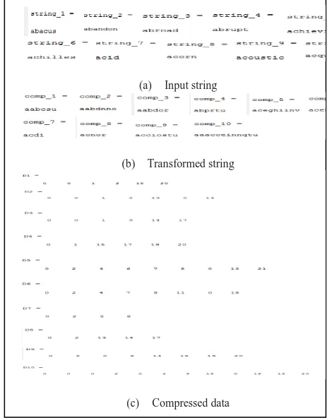
Consider the string of text: ‘abacus’, ‘abandon’, ‘abroad’, ‘abrupt’, ‘achieving’, ‘achilles’, ‘acid’, ‘acorn’, ‘acoustic’, ‘acquaintance’ [20]. Simulation is done using ‘MATLAB R2010a’ tool. First, Burrows-Wheeler Transform and Move-to-front coding is applied to the string of text, which is shown in Figure-1.

Fig -1: ‘Burrows-Wheeler transform’ and ‘Move-to-front coding’ for string of text

(a) Input string

(b) Transformed string

[image:3.595.312.547.425.721.2]

(4)

Page 273

The Table-1 shows that, number of bits required to

represent the compressed data is compressed to some extent by applying the data compression algorithm such as ‘Burrows-wheeler transform’ and ‘Move-to-front coding’. Then, this compressed data is clustered into number of cluster 2, 3 up to √71≈ 8 using Hierarchical clustering and DB index is calculated and plotted as shown in Figure-2.

Table -1: Compressions of String of Text

Original string

Number of bits required to represen t the string

Compressed data

Number of bits required to

represent the compress ed data

Abacus 6 bits aabcsu 6 bits

Abandon 6 bits aabdnno 5 bits

Abroad 6 bits aabdor 6 bits

Abrupt 7 bits abprtu 7 bits

Achieving 7 bits aceghiinv 6 bits

Achilles 6 bits acehills 5 bits

Acid 4 bits acdi 4 bits

Acorn 6 bits acnor 6 bits

Acoustic 7 bits acciostu 7 bits

Acquaintane 7 bits aaacceinnqtu 7 bits

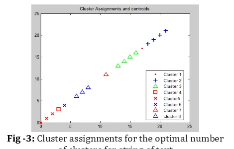
Figure-2 shows the plot of the DB index versus number of cluster, where at the number of cluster 8, we got the minimum value as 0.2070 which indicates that optimal number of cluster is 8. The cluster assignment is shown in Figure-3.

[image:4.595.320.555.170.320.2]

Figure-3 shows that data is clustered into eight clusters, where red colored dot symbol indicates the data elements of cluster 1, blue colored plus symbol indicates the data elements of cluster 2, green colored triangle symbol indicates the data elements of cluster 3, red colored square symbol indicates the data elements of cluster 4, red colored cross symbol indicates the data elements of cluster 5, blue colored cross symbol indicates the data elements of cluster 6, red colored triangle symbol indicates the data elements of cluster 7 and blue colored triangle symbol indicates the data elements of cluster 8.

Table -2: Comparison of the Execution Time of Algorithms With and Without Applying The Data Compression For

String of Text

Execution time

Clustering without compression

(seconds)

Clustering with compression(se

conds)

1.072108 0.971097

As shown in the Table -2, execution time of clustering the compressed data is less than clustering the original data (without compressing).

5.2 Case 2

In this case, K-means and Hierarchical clustering is compared. The result of the previous case that is, compressing and clustering of the string of text is compared with the result of clustering the same dataset by using the K-means clustering. Hence, first consider the Fig -2: Davies-Bouldin index versus no. of cluster for

the string data

[image:4.595.37.290.194.771.2] [image:4.595.311.558.516.621.2]

(5)

Page 274

string of text: ‘abacus’, ‘abandon’, ‘abroad’, ‘abrupt’,

‘achieving’, ‘achilles’, ‘acid’, ‘acorn’, ‘acoustic’, ‘acquaintance’ [20]. Figure-1 shows the compressed data of this string.

Then this compressed data is clustered into number of clusters 2, 3 up to √71≈8 by using K-means clustering. But here, for the number of cluster=8, it shows empty cluster so data is clustered up to Kmax=7 clusters and silhouette

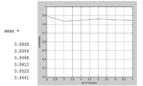
index is calculated for all the clusters to find the optimality. Then mean silhouette value is calculated and plot is shown in the Figure-4.

Figure-4 shows that, at the number of cluster 2, we got the maximum value as 0.8938 which indicates that optimal number of cluster is 2. Hence, if the data elements are clustered into two clusters, we get the compact and well separated a cluster which is shown in Figure-5.

Figure-5 shows that dataset is clustered into two clusters, where red colored dot symbol indicates the data elements of cluster 1 and blue colored plus symbol indicates the data elements of cluster 2. It takes 3.832 seconds of time to cluster the given dataset by using the K-means algorithm.

Table -3: Comparison of Algorithms

Algorithm Optimality Execution

time(seconds)

K-means 2 3.832

Hierarchical 8 0.971

Table-3 shows the comparison of the K-means and Hierarchical algorithm, which has following results

 Hierarchical algorithm clusters the data faster than the K-means algorithm.

 For the Hierarchical algorithm, we get optimality as 8 and where as in K-means for 8, we get the empty cluster and optimality at number of cluster = 2. Hence, Hierarchical clustering has good quality of cluster as optimality is 8.

 But, for the large datasets dendrogram of the Hierarchical clustering becomes very complex, that is, it is difficult to analyze the number of clusters and data elements that belongs to the clusters.

7. CONCLUSION AND FUTURE WORK

In this work the K-means algorithm is used to cluster the data points, Hierarchical algorithm is used to cluster the string of text and K-means and Hierarchical algorithms are compared. For clustering the string of text, compression algorithms such as ‘Burrows-Wheeler transform’ and ‘Move-to-front coding’ are used to compress the data, so that size of the data should be reduced to some extent. Implementation is done using ‘MATLAB R2010a’ tool and results are plotted. The performance measure of the algorithm is verified by using the validity indices such as ‘Silhouette index’ and ‘Davies-Bouldin index’.

Since data is collected from various networks. Hence, future work is to ‘Cluster the heterogeneous data collected from different types of network and reduce the time consumption’.

ACKNOWLEDGEMENT

I would like to express our deep sense of gratitude to our Principal Dr V.P.HUGGI for providing all the facilities in the college.

I would like to thank our H.O.D Prof. S.R.PUROHIT for providing us all the facilities and fostering congenial academic environment in the department.

I feel deeply indebted to our esteemed guide Prof. D.I.HATTI for her guidance, advice and suggestion given throughout the work.

Fig -4: Mean silhouette index versus number of clusters for the string of 10 words

[image:5.595.44.280.259.401.2] [image:5.595.43.254.515.678.2]

(6)

Page 275

I would like to take these opportunities to thank all the

faculty members and the supporting staff for helping us in this endeavor.

Not the last, but the least I would like to thank my parents, my husband and all my family members.

REFERENCES

[1] A. Alamri, W. S. Ansari, M. M. Hassan, M. Shamim Hossain, A. Alelaiwi and M. Anwar Hossain, A Survey on Sensor-Cloud: Architecture, Applications and

Approaches, International Journal of Distributed

Sensor Networks, vol. 2013, pp. 1-18, Nov. 2012. [2] Chandrani. Ray Chowdhury, A Survey on Cloud Sensor

Integration”, International Journal of Innovative

Research in Computer and Communication Engineering,

vol. 2, Issue 8, pp. 5470-5476, Aug. 2014.

[3] Fabian Nack, An Overview on Wireless Sensor Network, Institute of computer Science (ICS), University, Barlin, pp. 1-8.

[4] Jiawei Han, Micheline Kamber and Jian Pei, Data Mining Concepts and Techniques, 3rd _{edition, Aug.}

2000.

[5] A. K. Jain, M. N. Murty and P. J. Flynn, Data Clustering: A Review, ACM Computing Sueveys, vol. 31, no. 3, pp. 265-317, Sep. 1999.

[6] Dr. M. P. S Bhatia and Deepika Khurana, Experimental Study of Data Clustering using K- Means and Modified Algorithms, International Journal of Data Mining & Knowledge Management Process (IJDKP), vol. 3, no. 3, pp. 17-30, May 2013.

[7] Pavel. Berkhin, Survey of Clustering Data Mining Techniques, pp: 1-56, 2002.

[8] S. Anitha Elavarasi, Dr. J Akilandeswari and Dr. B Sathyabhama, A Survey on Partition Clustering

Algorithm, International Journal of Enterprise

Computing and Business System, vol. 1, issue. 1, pp. 1-13, Jan. 2011.

[9] Peter. Grabusts, The Choice of Metrics for Clustering Algorithms, 8th_{International Scientific and Practical}

Conference, vol. 2, pp. 70-76, 2011.

[10] T. M. Kodinariya and Dr. Prashant. R. Makwana, Review on Determining Number of Clusters in K-means Clustering, International Journal of Advance Research in Computer Science and Management studies, vol. 1, issue 6, pp. 90-95, Nov. 2013.

[11] U. Maulik and Sanghamitra Bandyopadhyay, Performance evaluation of some Clustering algorithm

and Validity indices, IEEE Transaction on pattern

analysis and machine intelligence, vol. 24, no. 12, pp. 1650-1654, December 2002.

[12] M. Burrows and D. J. Wheeler, The Block-sorting Lossless Data Compression Algorithm, Digital System Research Center, pp. 1-18, May 1994.

[13] M. Yuriyama and T. Kushida, Sensor Cloud infrastructure-Physical Sensor Management with

Virtualized Sensors on Cloud Computing, International Conference on Network-based information system (NBiS), IEEE, pp. 1-8, Sept 2010.

[14] Sajjad Hussain Shah, Fazle Kabeer Khan, Wajjid Ali and Jamsheed Khan, A new framework to integrate

wireless sensor networks with cloud computing,

Aerospace Conference, IEEE, pp. 1-6, March 2013

.

[15] M. Vijayalakshmi and M. Renuka Devi, A Survey of

Different Issue of Different clustering Algorithms Used in Large Data sets, International Journal of Advanced Research in Computer Science and Software Engineering, vol. 2, issue 3, pp. 305-307, March 2012. [16] Guojun Gan, Chaoqun Ma and Jianhong Wu, Data

Clustering: Theory, Algorithms, and Applications, ASA-SIAM Series on Statistics and Applied Probability, SIAM, Philadelphia, ASA, Alexandria, pp. 1-455, July 2007.

[17] Yanchi Liu, Zhongmou Li, Hui Xiong, Xuedong Gao and Junjie Wu, Understanding of Internal Clustering Validation Measures, 10th_{International Conference on}

Data Mining, IEEE, pp. 911 – 916, December 2010. [18] Olatz Arbelaitz, Ibai Gurrutxaga, Javier Muguerza,

Jesus M. Perez and Inigo Perona, An extensive comparative study of cluster validity indices, Pattern Recognition Journal, vol. 46, issue. 1, pp. 243-256, January 2013.

[19] www.tutorialspoint.com/matlab

[20] http://archieve.ics.uci.edu/ UCI Machine Learning Repository.

BIOGRAPHIES

Ms. Anjali J Rathod is a PG student in Digital Communication and Networking, Dept. of Electronics and Communication Engineering, B.L.D.E.A’s Engineering College, Vijayapur. My areas of interest are Sensor-Cloud and Data Clustering.

Mrs. Daneshwari I Hatti working as a Assistant Professor in Dept.

of Electronics and

Communication Engineering,

Analysis of Clustering Algorithms for Data Management in Sensor Cloud

Page 270