EMPLOYING SENSOR NETWORK TO GUIDE FIREFIGHTERS
IN DANGEROUS AREA
Hamidreza Koohi
Department of Computer Engineering, Shomal University, [email protected]
Ehsan Nadernejad*
Department of Photonic, Technical University of Denmark, B. 343, 2800 Lyngby, Denmark, [email protected]
Mahmoud Fathi
Department of Computer Engineering, University of Science and Technology [email protected]
*Corresponding Author
(Received: November 29, 2009– Accepted in Revised Form: March 11, 2010)
Abstract In this paper, we intend to focus on the sensor network applications in firefighting. A distributed algorithm is developed for the sensor network to guide firefighters through a burning area. The sensor network models the danger of the area under coverage as obstacles, and has the property to adapt itself against possible changes. The protocol developed, will integrate the artificial potential field of the sensors with the information of the intended place of moving firefighter so that it guides the firefighter step by step through the sensor network by choosing the safest path in dangerous zones. This protocol is simulated by Visual-Sense and the simulation results are available.
Keywords Firefighter, Sensor Network, Potential Field, Area’s Danger, Navigation.
ﻩﺪﻴﻜﭼ
ﻣﻦﻳﺍ ﺭﺩ
ﻘ ﻪﻟﺎ
ﺭﻮﮕﻟﺍﺖﺳﺍ ﻩﺪﺷﯽﻌﺳ
ﻳ
ﺯﻮﺗﯼﺎﻫﻢﺘ
ﻳ
ﺖﻬﺟﯽﻧﺎﻣﺯﺎﺳﺩﻮﺧﺭﻮﺴﻨﺳﯼﺎﻫﻪﮑﺒﺷ ﯼﺍﺮﺑ،ﯽﻌ
ﻥﺎﻴﻣﺯﺍﻥﺎﺸﻧﺶﺗﺁﺖﻳﺍﺪﻫ
ﻳ
ﺩﻮﺷﻩﺩﺍﺩﺵﺮﺘﺴﮔﯼﺯﻮﺳﺶﺗﺁﻪﻘﻄﻨﻣﮏ
.
ﻪﮐﺍﺭﯼﺍﻪﻘﻄﻨﻣﺮﻄﺧﺢﻄﺳ،ﺭﻮﺴﻨﺳﻪﮑﺒﺷ
ﺖﺤﺗ
ﺪﻫﺩﻖﻓﻭ ﯽﻟﺎﻤﺘﺣﺍﺕﺍﺮﻴﻴﻐﺗﻞﺑﺎﻘﻣﺭﺩﺍﺭﺩﻮﺧﻪﮐﺩﺭﺍﺩ ﺍﺭﺖﻴﻠﺑﺎﻗﻦﻳﺍﻭﺪﻨﮐﯽﻣﻝﺪﻣ،ﺩﺭﺍﺩﺶﺷﻮﭘ
.
ﻪﮑﺒﺷ
ﺪﻧﺎﻳﺎﻤﻧ ﯽﻣ ﻊﻧﺎﻣ ﻥﺍﻮﻨﻋ ﻪﺑ ﺍﺭ ﮎﺎﻧﺮﻄﺧ ﻖﻃﺎﻨﻣ ﺭﻮﺴﻨﺳ
.
ﺪﻠﻴﻓ،ﺖﻓﺎﻳ ﺪﻫﺍﻮﺧ ﺵﺮﺘﺴﮔﻪﻟﺎﻘﻣ ﻦﻳﺍ ﺭﺩ ﻪﮐ ﯽﻠﮑﺗﻭﺮﭘ
ﺩ،ﺖﮐﺮﺣﻝﺎﺣﺭﺩِﻥﺎﺸﻧﺶﺗﺁﻑﺪﻫﻥﺎﮑﻣﺕﺎﻋﻼﻃﺍﺎﺑﺍﺭﺎﻫﺭﻮﺴﻨﺳﯼﺯﺎﺠﻣﻞﻴﺴﻧﺎﺘﭘ
ﻥﺎﺸﻧﺶﺗﺁﺎﺗﺩﺰﻴﻣﺁﯽﻣﻢﻫﺭ
ﯽﻳﺎﻤﻨﻫﺍﺭﻡﺪﻗﻪﺑﻡﺪﻗ،ﺪﻨﻳﺰﮔﯽﻣﺮﺑﮎﺎﻧﺮﻄﺧﻖﻃﺎﻨﻣﺯﺍﺍﺭﻪﻠﺻﺎﻓ ﻦﻳﺮﺗﻦﻣﺍﻪﮐﯽﻟﺎﺣﺭﺩﺭﻮﺴﻨﺳﻪﮑﺒﺷﻥﺎﻴﻣﺯﺍﺍﺭ
ﺪﻨﮐ
.
1. INTRODUCTION
Fire causes far more victims compared to other natural disasters. For example, in the U.S.A about 1.9 million fires occurs annually which leave about 4000 fatalities and 2500 injuries. Likewise 100 firemen lose their lives in the line of duty. In addition fires inflict 11 million dollars damage on properties and installations [1].
Firemen generally conceptualize fire situations improperly. It is difficult to collect data at the time of fire because it requires firemen to enter into uncharted and dangerous areas. Currently
firefighters take little advantage of digital technology. Integrated computational technologies allow for the needed changes to the current practice. Electronic coverage is being developed for military use and Emergency services. Personal Protective Equipment (PPE) [2] for the firemen is an example of such electronic systems. These PPE's can be used to fit a mobile node of sensor network built-in the fatigues of a fireman in order to establish communication with the fixed nodes of sensor network.
sensor network researchers have studied more on protocols for different layers but less in its applications in real world. This paper endeavors to deal with the applying a sensor network in a firefighting process. Distributed Algorithms are developed for self organizing sensor networks to direct the firemen through a burning area. A series of operating sensors which have been networked together can follow the exciting movements of firemen in fire perimeter and direct them to desired spot.
This paper endeavors greatly to examine the theories laid down for networks allowing themselves to adjust to environments based on a plan depicting the environment risks by relying on important achievements that have been formerly undertaken [3-7]. By assuming dangerous places as obstacles we calculate the artificial potential field based on obstacles that will be in tune with current system's status. We then develop a distributed protocol that combines this artificial potential field with information about the direction and goal of the moving object and guarantees the best safest path to the goal. What we mean by the phrase "safest direction" is that it evades the least number of traces of danger. Similarly, we shall present a protocol to disseminate information through sensor network as well as roadmap to detect risks with the range of course. Visual sense software derived from the PtolemyII was used to simulate this protocol. As opposed to other simulation tools that handle protocol's support much further, this software allows us to address ourselves to sensor network applications.
2. RELATED WORK
We are inspired by previous work in sensor networks [8], ad-hoc networks [9-12] and Robotic [13, 14]. In [4] by using direct diffusion approach, the data generated by sensor nodes is named by attribute-value pairs. A node requests data by sending its interests for the named data. The interests will be propagated within the network to find the source of the related data. The direct diffusion method is used to reinforce the best path from the source to the sink. We propose to actively disseminate the information in the network, and
consider the sensor network as an information base.
In [3], the minimal exposure path problem in a sensor network is considered. That paper developed an efficient and effective algorithm for the problem. We consider a seemingly similar problem. We are concerned about the dangerous area rather than the coverage of an individual sensor. Instead of calculating the information about the worst case exposure-based coverage caused by the deployment of a sensor network, we use the sensor network to compute a path that can navigate a firefighter to the goal by avoiding dangerous area. Furthermore, we use distributed algorithms to disseminate the data in the sensor network.
There have been many studies conducted on Mote sensor network, especially in [3, 4] that are closely related to our system implementation. An empirical study on networks composed of over 150 Motes was conducted in [6]. The paper presents the data collected in different layers and reveals that even a simple protocol can exhibit a large complexity in the Mote network. It gives many very useful experimental data on a real sensor network platform. Some of the observations from our experiments show the same behaviors in many scenarios with [6, 7] papers.
Scaglione et el. [15] showed an approach to work around the vanishing per-node throughput problem by coupling routing and source coding in a sensor network. We use the number of hops to evaluate the distance between sensors as done in [16].
Jinyang et al. [19] have introduced a GLS. This is a scaleable distributed location service which tracks mobile node location. Allen K.L.M, in his thesis [20], refers to devising a CricketNav system as an indoor mobile navigation system. That requires user carrying a set such as a PDA for computation.
Discusses the use of an artificial potential field for robot motion planning. A robot moving in accordance to the potential will never hit obstacles, but it may get stuck in local minima. We combine these two methods to find the best path to the goal, which is safe and short, and modify them to exploit the distributed nature of sensor networks.
3. A DISTRIBUTIVE ALGORITHM FOR GUIDING NAVIGATION OF A
FIREFIGHTER
Sensors collect information from areas under their monitoring. They can store the information locally or route them to a base station for further analysis and use. Sensors can also use communicative facilities to integrate their sensed values with the rest of the sensor landscape. We will discuss a method to distribute the information about the environment redundantly across the entire network. Firemen can use this information as they traverse the network. They are also guided across the network along a safe path, away from the type of danger that can be detected by the sensors.
The dangerous areas in the sensor network will be defined as obstacles. Danger may include overheating, fire, hazardous gasses, thick fume, etc. It is supposed that each sensor can sense the presence or absence of such types of danger. A danger configuration protocol running across all the nodes of the network creates the danger map. We do not envision that the network will create accurate geometric map, distributed across all the nodes. Instead, we wish for the nodes in the network to provide some information about how far from danger each node is. If the sensors are uniformly distributed, the smallest number of communication hops to a sensor that triggers "yes" to danger is a measure of the distance to danger. The goal is to find a path for a fireman that avoids the dangerous areas. We envision having the user ask the network regularly for where to go next. The nodes within broadcasting range from the user supply the next best step.
In order to supply obstacle information to the planning algorithm we use artificial potential fields. In an artificial potential field, firefighters moves under the actuation of artificial forces.
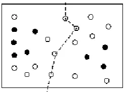
Usually, the goal generates an attractive potential which pulls the object to goal. The obstacles generate a repulsive potential which push the object away from the goal. The gradient of the total potential is the artificial force acting on the object. The direction of this force is the current best direction of motion. The obstacles that they correspond to dangerous areas will have repulsing values; the goal will also have an attracting value. As shown in figure 1; in figure 1 the solid black circles show sensors that sense dangers and those of white are sensors that have not sensed it. The dashed line shows the guiding path across the area covered by the sensor network. It should be noted that this direction crosses from one sensor to another and preserves the maximal distance from areas of danger while approaching the exit point. Algorithm 1 shows the potential field protocol. The potential field is computed in the following way. Each node whose sensor triggers danger diffuses the information about danger to its neighbors in a message that includes its source node id, the potential value and the number of hops from the source of the message to the current node. When a node receives multiple messages from the same source node, it keeps only the message with the smallest number of hops. The message with the least hops is kept because that message is likely to travel along the shortest path. The current node will compute the new potential value from this source node. Then, the node broadcasts a message with its potential value and number of hops to its neighbors.
After this configuration procedure, nodes may have several potentials from multiple resources; to compute its current danger level information each node adds all the potentials.
It is to be noted that the potential field protocol provides distributed repository of information about the area covered by the sensor network. It can be applied in an initialization phase, continuously or intermittently. The sensor network can self organize adaptively to the current landscape. It updates its distributed information content by running the potential field computation protocol regularly. In this way, the network can adapt to sensor failure and to dynamic danger sources that can move across the network.
The potential field information stored at each node can be used to guide firemen equipped with a sensor that can establish an online interaction with the network. The safest path to the goal can be computed by using protocol 2. The goal node initiates a dynamic programming computation of
this path using broadcasting. The goal node broadcasts a message with the danger degree of the path, which is zero for the goal. When a sensor node receives a message, it adds its own potential value to the potential value provided in the message, and broadcasts a message updated with this new potential to its neighbors. If a node receives multiple messages, it selects the message with the smallest potential (corresponding to the least danger) and remembers the sender of the message.
A firefighter in the sensor network can rely on the information computed using Algorithms 1 and 2 to get continuous feedback from the network on how to traverse the area. Algorithm 3 shows the navigation guiding protocol. The firefighter asks the network for where to go next. The neighboring nodes reply with their current values. The firefighter's sensor chooses the best possibility from the returned values. Note that this algorithm requires the integrated potential computed by Algorithms 1 and 2 in order to avoid getting stuck in local minima.
3.1 IMMLEMENTATION
Our navigation algorithms have an implicit assumption that the communication paths in the network are bi-directional. Since the safest path is computed backward from the goal, messages have to be able to flow in the opposite direction to lead the user to the goal. However, all attachments are not always manipulated as bi-directional in sensor networks. For example see Figure 2 that shows the distribution of symmetric and asymmetric links in Algorithm 1: The potential field computation
protocol.
1: for all sensors Si in the network do 2: pot = 0i , hops = j ∞ for any danger j
3: if sensed-value = danger then 4:
i
hops = 0, pot = Infinity i 5: Broadcast message (i, hops = 0) 6: if receive (j, hops) then
7: if hopsjhops1 then 8: hopsjhops1 9: Broadcast message (j;
j
hops )
10: for all received j do 11: Compute the potential
j
pot of j using
2
1 j
j
hops
pot
12: Compute the potential at Si using all j
pot ,
i
pot = poti + j
pot
Algorithm 2: The safest path to goal computation protocol.
1: Let G be a goal sensor
2: G broadcasts msg = (G , id my (G), hops = 0, id
potential = 0)
3: for all sensors Si do
4: Initially
g
hops = and Pg=
5: if receive (g, k, hops, potential) then
6: Compute the potential integration from the goal to here:
7: if
i g potential pot
P then
8: Pgpotentialpoti 9: hops hops1
g
10: priorgk 11: Broadcast (
id
G , my (id S ),i hops ,g Pg)
Algorithm 3: The navigation guiding protocol. 1: if Si is a user sensor then
2: while Not at the goal G do 3: Broadcast inquiry message (Gid)
4: for all received messages m = (
id G , id my ( k S ),
hops, potential, prior) do
5: Choose the message m with minimal potential then minimal hops.
6: Let myid(Sk) be the id for the sender of this
message
7: Move toward
id
my (
k
S ) and prior.
8: if Si is an information sensor then 9: if receive (
id
G ) inquiry message then
10: Reply with (Gid,
id
my (S )i ,hopsg,Pg,priorg
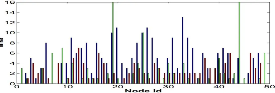
Figure 2: Distribution of symmetrical and asymmetrical links in one experiment.
an experiment with a 7*7 grid of Mote sensors, the x-axis shows the node id and the y-axis the number of links. Three bars have been designed for each node: the first shows the number of symmetric links, the second the number of unidirectional outgoing links and the third the number of unidirectional incoming links. This is consistent with data from [6]. This paper intends to use the following methodology to identify bi-directional links in a network. The computation can be thought of as an additional protocol run by each node.
Each node performs neighbor profiling to find all its stable one-hop neighbors bi-directionally; that is, these neighbors should be reachable to and from the node with high probability. In this way we may ward off the unidirectional link nodes that may lead to long distance hops. Each node only uses the received packets from its stable neighbors after profiling. In our current implementation, we perform the neighbor profiling on the fly. Every time a node receives a packet, it increases the frequency of the sender of the packet, which measures the stability of that link. A link is used only if its frequency is higher than some threshold value, which is one fifth of the maximal frequency of all the links in our implementation. 1/5 is a parameter we chose for our experiments.
A side effect of neighbor profiling is the removal of many of the transient links that are active for a very short time. By exchanging the information about the frequency of two neighbors, the system ends up using the most stable
bi-directional links. Our hop distance can also be close to the average instead of being too abnormal. Algorithms 1 and 2 ask each sensor upon receiving a message to broadcast with fewer hops to the dangerous area or with a smaller potential integration to the goal. Many of the broadcasts may not be necessary since only the message with the least hops to the danger node location or the minimal potential integration to the goal is useful. To reduce the message broadcasts, we let each sensor wait for some time before it broadcasts. The waiting time for sensor Si is proportional to one unit in Algorithm 1 and the value poti in
Algorithm 2. The main idea is to let the message traveling time be proportional to the hops from the danger or the potential integration along the path traveled. Therefore only the messages that carry the optimal value will be broadcasted and those carrying the non-optimal value will be suppressed. We can prove that the number of message broadcasts for each sensor is 1 in each algorithm using this technique [21]. In our current implementation, we let each sensor wait for one time unit plus a small random time to reduce the message broadcasts and traffic congestions due to the simultaneous transmissions.
handle the incoming packets. Thus it is important that we design protocols that repeat the packet transmission. Most of the information stored at a node can be inferred by reading the protocols. To adapt the network topology change, each sensor can periodically flush its route cache (route to obstacles and goal) with all the other information unchanged. Currently we have not included the capability to tune the cache expiration timer.
3-2 ANALYSIS OF PROTOCOL 3-2-1 ACCURACY OF PROTOCOL
Our protocols can correctly determine the safest path to the goal without getting stuck in the local minima that are often an issue with artificial potential field methods.
Theorem 1: Algorithm 3 will always give the firefighter sensor a path to the goal.
Proof: In Algorithm 2, the prior link of a node points to a node that has potential value less than that of the current node. So for each node other than the goal, there must be a neighboring node that has a smaller potential value. This proves that there are no local minima in the network.
The fire fighter's sensor can always find a node among its neighbors that leads to a smaller potential value. If the process continues, the node will end up with the goal that has the smallest potential value 0. Therefore, Algorithm 3 can always give the firefighter sensor a path to the goal.
3-2-2. THE HOP DIISTANCE MODEL
One critical assumption behind Algorithm 1 is that we can represent distance in terms of numbers of hops. In general, how realistic is this model? To answer this question, we consider how the density of the sensor distribution affects the distance evaluation in our algorithms. We now address this question for the case when each node has a constant transmission range, which is an assumption consistent with the test bed hardware. The key metric is the minimal number of hops between any two sensors that are distance apart. Since in our algorithms each sensor uses flooding to broadcast packets to all of its neighbors and each sensor within the transmission range of the broadcasting sensor can forward the packets, it is very hard to characterize this metric. An
approximation can be obtained by allowing only the sensors at the boundary of the transmission range to forward packets. Of all those sensors we choose the sensor that can make the most progress in the direction of the destination sensor. The number of hops computed this way is an approximation of the minimal number of hops. In [22], Takagi et el proposed the multi direction forward routing and analyzed its average progress in the direction of the destination. We can use the same analysis to approximate the distance of a single hop.
Based on the analysis in [22], suppose that '
R is
the average progress and R is the transmission
range. Then the minimal ideal hops should be R,
but the expected minimal hop in our real sensor network is '
R
. That is, the distance we evaluate is always '
R
R times of the real distance.
In [6], Ganesan et al. reported the length of a hop may not be fixed, as we observed in our experiments. By experiments, we can get the expectation and the deviation of the length of a hop (call them E and d). According to central limit
theorem in probability theory, the length of n hops
has the expectation of nE and the deviation of nd
, that is, the deviation between the real distance and the computed distance is in the order of nd,
which is small compared with the distance of the order of nE. This actually shows that our
algorithms are robust in the real network scenario.
3-2-3: PERFORMANCE BOUND OF THE COMPUTED PATH
We expect our protocols to compute the integrated potential value on the safest path, but the
implementation introduces error. We can compare the integrated potential value on the path found by our protocols and the optimal path to show how safe the found path would be.
Theorem 2: The computed potential integration on the computed path is upper and lower bounded with respect to the actual potential integration on the path.
In theory, there is an optimum path with the least value of potential integration and may not traverse any sensor node. But this path is not feasible in our system since a user can only go from one sensor to another by listening to the reply from the next sensor in our navigation protocol. Therefore, instead of designating an optimal path, the introduced protocols can determine an optimal sensor path as one that is composed of a series of sensor nodes that are connected consecutively by straight line segments (the connected nodes are within the transmission range of each other), which we expect to characterize the motion of a user. Theorem 3: The potential integration on the computed path is upper bounded with respect to the potential integration on the optimal sensor path. This theorem has also been suggested and demonstrated by Li et al. [7]. According to this theorem the computed path is limited by potential integration.
3-2-4: PROPAGATION AND
COMMUNICATION CAPABBILITIES
Two natural questions arise about the protocols we described previously: How much time does it take to propagate the obstacle and goal information? Is the network capable of transmitting all the information? In this section, we answer the two questions in the context of our current implementation, in which we use one packet for propagating the information of each obstacle or goal for every broadcast. To optimize the bandwidth usage by reducing the information transmission, we can combine the information about two or more obstacles and the goal into a packet, or use information encoding to reduce the information redundancy among the neighboring nodes. It is no surprising they can provide performance gain to our system.
We assume that each node has fixed transmission range and the nodes in a node's neighborhood (say k nodes) should be silent to avoid contention when that node broadcasts. For the obstacle information propagation, assume the number of the concerned obstacles is o; i.e., on
average, each node has to process the information of o obstacles. Let the transmission rate for each node be bpackets s. Then the time for the obstacle
information propagating to a node is okl b where
Llolmin , , L is the distance for the potential
value to become zero, and lo is the distance between the node and the obstacle, both in number of hops. The formula is for the case when we add waiting time for each broadcast; i.e., each node only broadcasts once for each obstacle information propagation. In this case, each node needs to wait for k btime before broadcasting the best value.
This waiting time allows enough time for each of the node's neighbors to broadcast the packet if they hold the same value as this node, so that they do not collide. For the case without explicit waiting time scheme, the MAC protocol enforces this delay to make sure all the packets go through smoothly. On the other hand, suppose we do not have the waiting time scheme, each node may broadcast multiple times because the least number of hops is unlikely to be obtained by the first received message so that the node needs to broadcast several packets before the best value is propagated. In this case, we must multiply the propagation time by another parameter m, which is the average
messages broadcast for each node. Similarly, we can evaluate the propagation time for the goal information.
The transmission rate of the some Mote sensors is approximately b=40packets s, so for k=8, the
added waiting time to each node is8400.2s.
Regardless of how many obstacles there are in this system, if each node is in the proximity of only one obstacle, it takes 0.2*10=2 seconds to propagate
the information up to 10 hops away. When the obstacles are static, and we do not care about the time, the network is capable of transmitting this amount of bits. If we have some constraints on the time, say, we have moving obstacles and the location of an obstacle must be known to the network within a distance resolution d, the network
may not be able to carry all the information. Suppose the maximal speed of the obstacle is v. In
the worst case, an obstacle generates v d packets
per time unit, so each node needs to process ov d
packets, which should be less thatb k, i.e., k
b d
ov . If we do not have the waiting time, we
Suppose a flame of fire is moving at a speed of 1m s, the maximal transmission rate for a node is
40packets s, the number of concerned obstacles is
1, and the number of the concerned neighbors of a node is 8. The network can sustain updates at a resolution of 0.2 meters. If we have the same network, but the moving object is a vehicle moving at a speed of 30miles h, the vehicle updates can
happen every 2.7 meters.
4. IMPLEMENTATION
Visual-Sense [23] from Ptolemy II simulation software package was used for simulation.
4.1 CORRECTNESS VALIDATION
Algorithms 1, 2 and 3 were simulated by using Visual-Sense. In simulation, we asked both the goals and the obstacles to generate the potential field and propagate it to the entire network periodically. This demonstrates experimentally that the goals and the obstacles can be added to the network at any time.
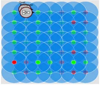
The goal is represented with a composite-wireless-actor. The nodes in the network that can sense the danger (obstacle) are represented with components that have two concentric circles where internal white circle represents node and external blue circle represent transmission range (see figure 3). The firefighter who moves in the network is represented with another component.
A grid containing 7*7 nodes was used to simulate experimenting the performance and accuracy of protocols. These nodes were deployed symmetrically and all neighbors are within communication range. The application is run by iterating a request for the next step by the user, a response by the network, and a move to the direction of the network response. To implement this last part we assume that the nodes know their location and that it can be transmitted to the moving user. This can be done by augmenting nodes with a GPS location, or via triangulation. Since we have not done this augmentation of the hardware yet, we simulate location knowledge by
placing the nodes in a grid pattern and supplying coordinates. The potential field and goal path computations are run by the network continuously.
When an obstacle or goal broadcasts, the receiving network node checks its list of known goals, and replaces the old data with the new broadcast if the new broadcast has a lower hop count. When a node receives a broadcast, it degrades the value of the broadcast based either on a linear function on the number of hops for goals or by the number of hops squared for obstacles. If the new value is not below a cutoff threshold, the packet is transmitted
Figure 3: Simulation with 7*7 sensor nodes in a network by means of Visual-Sense
to its neighbors. When a user requests potential estimates, all nodes that can hear it respond. The user chooses the node with the lowest value (that is lower than the value of the current node). The user moves toward this node.
This Simulation proved that a user with a sensor node actually went around the obstacles and got to the goal, via the correct path. We observed that the network adapted to the introduction of new obstacle nodes quickly and robustly.
When a new obstacle is inserted in the network, the obstacle starts broadcasting its danger information which affects the information held by each node. At this point Algorithms 1 and 2 cause the local information to change. We call the total time for the network to identify the new distances from danger and to the goal for each node the
“time for the network to stabilize”. In other words,
the time for the network to stabilize is the information propagation time in the network, which depends on the maximal hops from the goals or the obstacles to any node in the network. When an obstacle is added to the system online, it takes an identical amount of time to diffuse the information to the whole network.
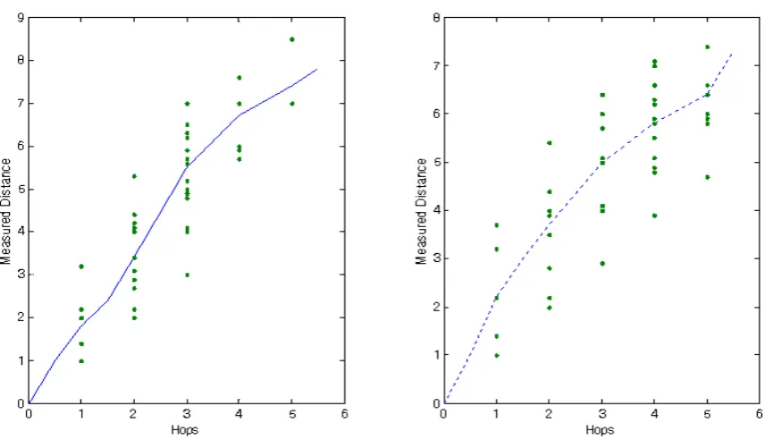
Figure 5 shows the comparison between the measured real distance and the hops counted using
our algorithm. The data was collected in our 7x7 grid network. We can see that the measured real distance is approximately linear in the number of hops.
4.2 SOME NOTES ON HARDWARE IMPLEMENTATION
Several interesting aspects of these experiments can be observed. The time for network stabilization (that is, the time for all the nodes to get the shortest distance to the danger source and the time for all the nodes to get the safest path to the goal) takes much longer than we expected. In our algorithms we made two typical assumptions: (1) a node broadcasts the message received immediately and (2) each node gets the packet traveling through the shortest path. We observed that on the hardware test bed neither of these assumptions was held. The network stabilization takes a long time because of network congestion and transitory link status. Often, nodes seemingly out of range hear each other for brief moments of time.
It seems that the following items are within the bounds of hardware implementation:
2. Asymmetric connection. It is observed that the transmission range in one direction may be quite different from that in the opposite direction. Thus, the assumption that if a node receives a packet from another node, it can send back a packet is too idealistic. In routing algorithm design, the existence of a route that can carry a packet from the source to a node does not guarantee a reverse route from that node to the source.
3. Congestion. Network congestion is very likely when the message rate is high. This is aggravated when the nodes in proximity of each other try to send packets at the same time. For a sensor network, because of its small memory and simplified protocol stack, congestion is a big problem.
4. Other unpredictable network conditions. In our sensor networks nodes that should be several hops away from each other occasionally come in direct communication range. We expect many transitory links (on and off) in an unstable network due to the impact of unpredictable conditions. We conclude that the uncertainty introduced by data loss, asymmetry, congestion, and transient links is fundamental in sensor networks. We need new models, algorithms, and simulations that take this kind of uncertainty into account. Guided by these lessons, we are currently conducting experiments to characterize better the likelihood of these uncertainty conditions.
5. SENSOR NETWORK AS A DISTRIBUTED INFORMATION REPOSITORY
Section 3 provided an example for how to use a sensor network as a distributed information repository about the environment in the context of a navigation guiding application. In this section we examine in more detail how to represent the information needed by our algorithm effectively in a sensor network. We thus examine the use of a sensor network as a distributed information repository.
Consider again the navigation guiding application formulated as a motion planning problem. Suppose multiple goals are installed in
the network. It is possible that each sensor has enough memory to store all the pertinent information about these goals. However, the current sensor hardware has very limited memory which restricts the amount of information that can be stored. We argue that sensors do not have to store all the information about the goals. Instead, all the necessary information should be stored somewhere, but not everywhere, in the network. The important thing is being able to retrieve the information any time it is needed.
Many sensors can cooperate to store information by having each sensor locally store only part of it. If the density of the network is such that multiple sensors cover the same area, the local information is the same for the sensors in some neighborhood. Thus, it does not matter who stores what. We propose that when a node receives a piece of information about the network, it randomly chooses to either keep it or to discard the information. To make this work, we must address (1) how to quantify the probability of discarding the information with respect to the information amount, the message size, and the density of the nodes; (2) how to retrieve the information from this sensor proximity, and (3) what are the tradeoffs between the memory utilization and broadcasting amount.
In order to address the information storage question, consider the proximity area S covered by
a group of sensors. All local (environmental) information about S is the same for all these
sensors. To use Algorithm 3, at least one of the sensors in S must store information about the goals. Let .S be the number of sensors in the area
where is the density of the sensor distribution and S is the area of the field in question. Suppose
each sensor has memory m. Then mS is the total
memory across all sensors. Let the amount of information to be recorded be
miwhere mi is thesize of information i. If ms
mi, then it ispossible that in the proximity area S, all the
required information can be found locally using Algorithm 3. To achieve this information distribution when the amount of information is too large for a node's memory (that is,m
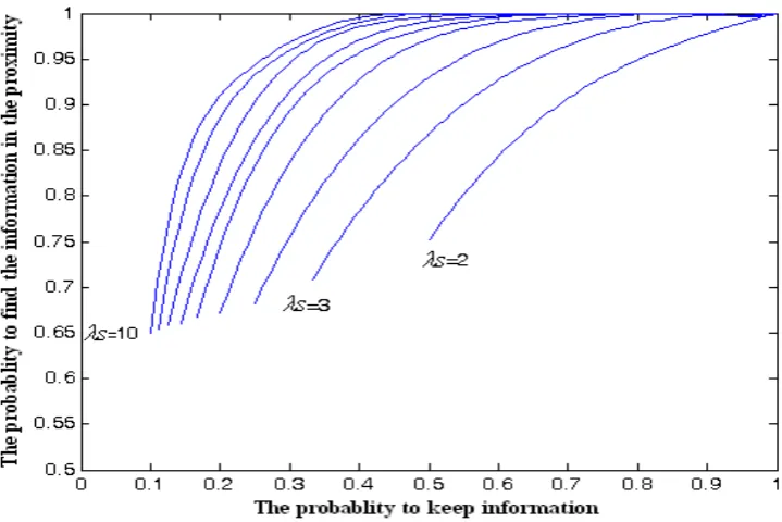
mi), weFigure 6: The probability (Y-axis) that a piece of information can be found in S, some neighborhood of a sensor. The X-axis is the probability that the sensor keeps a piece of information
information with probabilitypm
mi. When itreceives a piece of information, the probability that the information can be found in this area is
p
s1
1 (see Figure 6). In figure 6 we plot for
various numbers of sensors in the area from .S =
2 to .S = 10 where .S is the number of sensors
in that area. As the number of the sensors increases, the probability to find some information in that area is close to 1 even though the probability that a sensor keeps the information is small.
Another protocol can be implemented for locating a piece of information in a sensor network. If the information can not be found in the proximity area S, the sensor must try to retrieve
information beyond the area in the sensor network. Intuitively, the request for information is broadcast to all the sensors in the area S. The sensors who
have the information reply to the request. If there is no reply in the transmission range, the request must be broadcast again to a larger area, by making larger and larger concentric communication bands. More specifically, the user sends out the information request; the sensors in the broadcast range hear the request and reply if they have the
information. Otherwise no sensor replies to the request. After some period of silence with no reply (, the transmission time for the request and reply message), the user's requesting node sends out an information request for two hops. Each node receiving this message will broadcast the request out. If the information is found, it is sent back to the requesting node. Otherwise after some time of silence time with no reply for example2, the requesting node sends out an information request for three hops, and so on, until finally the information gets back to the requesting node.
6. CONCLUSION
the area of the network in the safest path. Safety is measured as the distance to the sensors that detect danger. Several protocols for solving this problem were described. Protocols presented implement a distributed repository of information that can be stored and retrieved efficiently when needed. We have used ideas from robotics to provide a correct solution to the navigation guiding task. We have simulated these protocols on a network of 7×7 sensor nodes by using the Visual-Sense software from Ptolemy II package.
The key metric used in our experimental evaluations is the time it takes the network to adapt to a new situation (detecting a moving object, detecting a new obstacle, adding a new sensor in the network, removing a sensor from the network, etc.). Our experimental work has taught us a number of lessons about some typical assumptions for designing protocols and has pointed out some important new directions of research.
7. REFERENCES
1. Jiang, X., Chen, N, Y,. Hong, J, I., Wang, K., Takayama, L., Landay, J, A.,“Siren: Context-aware Computing for Firefighting”, DUB Group, Computer Science and Engineering, University of Washington, Vol. 3001, (2004), 87-105.
2. Masterman, M, F., Leonhardt, D, T., Dunn, G, A., “Design of a Wearable Electronics Package for Firefighter Monitoring”, Proceeding of the Advanced Personal Protective Equipment Conference, (2005).
3. Meguerdichian, S., Koushanfar, F., Qu, G., Potkonjak, M,. “Exposure in wireless ad hoc sensor networks”. In MOBICOM, (2001), 139-150.
4. Intanagonwiwat, C., Govindan, R., Estrin, D., “Directed diffusion: A scalable and robust communication paradigm for sensor networks”. In Proc. Of Mobicom,
Boston, (2000).
5. Ye, F., Luo, H., Cheng, J., Lu, S., Zhang, L., “A two-tier data dissemination model for large-scale wireless sensor networks”. In ACM Mobicom, Atlanta, GA,
(2002).
6. Ganesan, D., Estrin, D., Woo, A., Culler, D., Krishnamachari, B., Wicker, S., “Complex Behavior at Scale: An Experimental Study of Low-Power Wireless Sensor Networks”, In UCLA Computer Science Tech, Report 02-0013, (2002).
7. Li,Q., De Rosa, M., Rus, D.,“Distributed Algorithms for Guiding Navigation across a Sensor Network”,
MobiCom ’03, (2003), San Diego, California, USA.
8. Estrin, D., Govindan, R., Heidmann, J., “Embedding the internet”, Communications of ACM, Vol. 43(5),
(2000),39-41.
9. Johnson, D, B., Maltz, D, A., “Dynamic source routing in ad-hoc wireless networks”, Mobile Computing, (1996), 153-181.
10. KO, Y, B., Vaidya, N, H.,“Location-aided routing (LAR) in Mobile ad-hoc networks”, In proceeding of ACM MobiCom, (1998), 66-75.
11. Murthy, S., Garcia-Luna-Aceves, J, J., “An efficient routing protocol for wireless networks”. ACM/Baltzer, MANET,Vol. 1(2), (1996),183-197.
12. Royer, E., Toh, C, K., “A review of current routing protocols for ad hoc mobile wireless networks”. In IEEE Personal Communication, Vol. 6, (1999), 46 – 55.
13. Corke,P., Hrabar,S., Peterson,R., Rus,D., Saripalliand, S., Sukhatme, G., “Autonomous Deployment and Repair of a Sensor Network using an Unmanned Aerial Vehicle”,IEEE International Conference on Robotics and Automation (ICRA), New Orleans, USA, (2004).
14. Latombe ,J, C., “Robot Motion Planning”, Kluwer, New
York, 1992.
15. Scaglione, A., Servetto, S., “On the Interdependence of routing and data compression in multi-hop sensor networks”, In ACM Mobicom, Atlanta, GA, 2002.
16. Nagpal, R., Shrobe, H., Bachrach, J., “Organizing a global coordinate system from local information on an ad hoc sensor network”. In IPSN LNCS 2634, (2003),
333-348.
17. Lengyel,J., Reichert, M., Donald, B., Greenberg, D., “Real-time robot motion planning using rasterizing computer graphics hardware”. In Proc. SIGGRAPII,
(1990), 327-336.
18. Koditschek, D, E., “Planning and control via potential functions”. Robotics Review I (Lozano-Perez and Khatib, editors), (1989), 349-367.
19. Li, J., Jannotti,J., De Couto, D, S, J., Karger,D, R., Morris,R., “A Scalable Location Service for Geographic Ad-Hoc Routing”, M.I.T. Laboratory for Computer Science, (2001).
20. Ka, A., Miu, L., “Design and Implementation of an Indoor Mobile Navigation System”, Master of Science Thesis in Computer Science and Engineering at the MIT, (2002).
21. Aslam, J., Li, Q., Rus, D., “Three power-aware routing algorithms for sensor networks”, Wireless
Communication and Mobile Computing, Vol. 3(2),
(2003),187-208.
22. Takagi, H., Kleinrock, L., “Optimal transmission ranges for randomly distributed packet radio terminals”. IEEE Transactions on Communications, Vol. 32(3), (1984),
246-257.
23. Baldwin, P., Kohli,S., Lee, E, A., Liu, X., Zhao, Y., “Modeling of Sensor Nets in Ptolemy II”, In Proc. of Information Processing in Sensor Networks, (2004),