Selecting Attribute to stand out in the Competitive World

Selecting Attribute to stand out in the Competitive World

Mr. Murlidher Mourya

, Mr. P.Krishna Rao

*

Computer Science, Vardhaman College of Engineering

**

Computer Science, Vardhaman College of Engineering

Abstract- Mining of frequent item sets is one of the most fundamental problems in data mining applications. My proposed algorithm which guides the seller to select the best attributes of a new product to be inserted in the database so that it stands out in the existing competitive products, due to budget constraints there is a limit, say m, on the number of attribute that can be selected for the entry into the database. Although the problems are NP complete. The Approximation algorithm are based on greedy heuristics. My proposed algorithm performs effectively and generates the frequent item sets faster.

Index Terms- Association rules,Data mining, Mining frequent itemsets.

I. INTRODUCTION

n recent years there has been development of ranking functions and efficient top-k retrivel algorithms which help the users in mining Frequent itemsset which plays a major role in many data mining applications .examples include: users wishing to search databases and catalogs of products such as homes, cars, cameras, or articles such as news and job ads. Users browsing these databases typically execute search queries via public front-end interfaces to these databases. Typical queries may specify sets of keywords in case of text databases or the desired values of certain attributes in case of structured relational databases. The query answering system answers `such queries by either returning all data objects that satisfy the quer conditions, or may rank and return the top-k data objects, or return the results that are on the query’s skyline. If ranking is employed, the ranking may either be simplistic—e.g., objects are ranked by an attribute such as Price; or more sophisticated—e.g., objects may be ranked by the degree of “relevance” to the query.

Attributes selection:

There are two types of users of these databases. Buyers of products who search such database trying to locate objects of interest ,while the latter type of user are sellers of products who insert new objects into these databases in the hope that they will be easily discovered by the buyers i.e it must stands out in the existing competitive products. To understand it a little better consider the following scenario : If a real estate seller wants to give an add on the news paper about sale of flats, He has to choose the best features of the flats, that are the most of the customers are interested. If he has given an add with some features (or attributes), and if no customer is interested on those features, then the add may not add value to his advertisement .If he has a system, that can suggest top k attributes (or features) of the product, then he can give a very good add, and that add will be referred by more number of customers. General problem also

arises in domains beyond e-commerce applications. For example, in the design of a new product, a manufacturer may be interested in selecting the 10 best features from a large wish-list of possible features—e.g., a homebuilder can find out that adding a swimming pool really increases visibility of a new home in a certain neighborhood. The problem here is selecting the proper and the best attributes of the flats, to give a good advertisement that is more number of customers areinterested.

To define our problem more formally, we need to develop a few abstractions. Let D be the database of products already being advertised in the marketplace (i.e .,the “competition”). let Q be the set of search queries that have been executed against this database in the recent past—thus Q is the “workload” or “query log.” The query log is our primary model of what past potential buyers have been interested in. For a new product that needs to be inserted into this database, we assume that the seller has a complete “ideal” description of the product. But due to budget constraints, there is a limit, say m, on the number of attributes/keywords that can be selected for entry into the database. Our problem can now be defined as follows.

II. PROBLEM FRAMEWORK

Given a database D, a query log Q, a new tuple t, and an integer m, determine the best (i.e., top-m) attributes of t to retain such that if the shortened version of t is inserted into the database, the number of queries of Q that retrieve t is maximized.

PRELIMINARIES

First we provide some useful definitions

Boolean database

Let D = {t1 . . . tN} be a collection of Boolean tuples over the attribute set A = {a1 . . . aM}, where each tuple t is a bit-vector where a 0 implies the absence of a feature and a 1 implies the presence of a feature. A tuple t may also be considered as a subset of A, where an attribute belongs to t if its value in the bit-vector is 1.

Table 1: Database

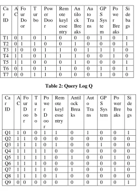
Table 2: Query Log Q

Ca r ID A C Fo ur D oo r T u r b o Po we r D oo r Rem ote keyl esse ntry Antil ock Brea ks Aut o Tra ns GP S Sys tem Po wer Bre aks Si de ba gs

Q1 1 0 0 1 1 0 1 0 0 1

Q2 1 1 0 0 0 0 0 0 0 0

Q3 1 1 1 0 1 0 0 1 0 0

Q4 1 1 1 1 0 0 0 0 0 0

Q5 1 1 1 1 0 1 0 0 1 0

Q6 1 1 1 0 0 0 0 0 0 0

Q7 1 1 1 1 0 1 0 0 1 0

Q8 1 1 1 0 1 0 0 0 0 0

Q9 0 0 0 0 0 0 0 0 0 1

Table 3: New Tuple T to be inserted

Ca r ID A C Fo ur D oo r T u r b o Po we r D oo r Rem ote keyl esse ntry Antil ock Brea ks Aut o Tra ns GP S Sys tem Po wer Bre aks Si de ba gs

T 1 1 1 1 0 0 0 0 0 0

Tuple domination.

Let t1 and t2 be two tuples such that for all attributes for which tuple t1 has value 1, tuple t2 also has value 1. In this case, we say that t2 dominates t1.

Tuple compression.

Let t be a tuple and let t’ be a subset of t with m attributes. Thus, t’ represents a compressed representation of t. Equivalently, in the bit-vector representation of t, we retain only m 1s and convert the rest to 0s. Query log. Let Q = {q1 . . .qS} be collection of queries where each query q defines a subset of attributes. The following running example will be used throughout the paper to illustrate various concepts

Conjunctive Boolean - Query Log (CB-QL): Given a query log Q with Conjunctive Boolean Retrieval semantics, a new tuple t, and an integer m, compute a compressed tuple t′ having m attributes such that the number of queries that retrieve t′ is maximized. Intuitively, for buyers interested in browsing products of interest, we wish to ensure that the compressed version of the new product is visible to as many buyers as possible.

Selecting the threshold value:

There are two alternate approaches to setting the threshold. One approach is essentially a heuristic, where we set the threshold to a reasonable fixed value dictated by the practicalities of the application. threshold enforces that attributes should be selected such that the compressed tuple is satisfied by a certain minimum number of queries. For example, a threshold of 1 percent means that we are not interested in results that satisfy less than 1 percent of the queries in the query log.

III. RELATED WORK

A large corpus of work has tackled the problem of ranking the results of a query. In the documents world, the most popular techniques are tf-idf based ranking functions, like BM25, as well as link-structure-based techniques like Page Rank if such links are present (e.g., the Web). In the database world, automatic ranking techniques for the results of structured queries have been proposed. Also there has been recent work on ordering the displayed attributes of query results.

Both of these tuple and attribute ranking techniques are inapplicable to our problem. The former inputs a database and a query, and outputs a list of database tuples according to a ranking function, and the latter inputs the list of database results and selects a set of attributes that “explain” these results. In contrast, our problem inputs a database, a query log, and a new tuple, and computes a set of attributes that will rank the tuple high for as many queries in the query log as possible.

Although the problem of choosing attribute is related to the area of feature selection,our work differs from the work on feature selection because our goal is very specific—to enable a new tuple to be highly visible to the database users and not toreduce the cost of building a mining model such as classification or clustering.

PINCER SEARCH ALGORITHM

Most of the algorithms used for mining maximal frequent itemsets perform fairly well when the length of the maximal frequent itemset is small. However, performance degrades when the length of the maximal frequent itemset is large, since in the bottom-up approach, the maximal frequent itemset is obtained only after traversing all its subsets.

The Pincer-search algorithm (Lin and Kedem, 1998, 2002), proposes a new approach for mining maximal frequent itemsets. It reduces the complexity by combining both top-down and bottom-up methods for generating maximal itemsets. The bottom-up search starts from 1-itemset and proceeds upto n -itemsets as in Apriori while the top-down search starts from n- itemsets and proceeds upto 1 itemset. Both bottom-up and top-down searches identify the maximal frequent itemsets by Ca r ID A C Fo ur Do or T ur bo Pow er Doo r Rem ote keyl esse ntry An tilo ck Bre aks Au to Tra ns GP S Sys te m Po we r Bre aks Si de ba gs

T1 0 1 0 1 0 0 0 1 0 1

T2 0 1 1 0 0 1 0 0 0 1

T3 1 0 0 1 1 0 1 1 1 0

T4 1 1 0 1 1 1 0 0 1 0

T5 1 1 0 0 0 1 0 0 0 1

T6 0 1 0 1 1 0 0 1 0 1

examining its candidates individually. Bottom-up search moves one-level up during a single pass whereas top-down search moves many levels down during a single pass. During the execution, all the itemsets are classified into 3 categories Frequent: Itemsets whose support is greater than min_sup are classified as frequent Infrequent: Itemsets whose support is less than min_sup are classified as infrequent Unclassified: All other Itemsets are said to be unclassified.

The Pincer algorithm is illustrated for the sample data source given in Table 4. The same data source will be used later for illustrating the proposed algorithm. An example of pincer search is shown in figure 1.

Pincer algorithm uses the following two properties to classify the unclassified itemsets Property 1: If an itemset is infrequent, all its supersets must be infrequent and they need not be examined further Property 2: If an itemset is frequent, all its subsets must be frequent and they need not be examined further

Table 4: Sample data source

The proposed work describes a novel method for generation of the maximal frequent itemsets with minimum effort. Instead of generating candidates for determining maximal frequent itemsets as done in other methods (Lin and Kedem, 2002), this method uses the concept of partitioning the data source into segments and then mining the segments for maximal frequent itemsets. It thus reduces the number of scans over the transactional data source to merely two. Moreover, the time spent for candidate generation is eliminated.

This algorithm involves the following steps to determine the MFS from a data source.

1.Segmentation of the transactional data source. 2. Prioritization of the segments

3. Mining of segments

TID ITEMS

T1 a,d,e,g,j

T2 a,b

T3 a,b,c,e,h

T4 a,b,c,d

T5 a,b,c,d,f,i

T6 a,b,c

T7 a,b,c,d,f,i

T8 a,b,c,e

Segmentation involves dividing the data source into a number of equal-sized segments. After segmenting, the segments are prioritized based on its support count (horizontal count). Once the priority is set, the segments are mined for maximal itemsets in the order of their priority. These steps are discussed in detail below.

Segmentatiom of the Transactional data source

The transactional data source is divided into a number of equal-sized segments. The segment size can be determined depending on the minimum threshold, min_sup.

Number of equal-sized segments ≤ 100 ---

Min_sup %

With such partitioning, the number of transactions in a segment will not be less than min_sup % of the total transactions, |D|. Each segment is associated with a new data structure called Item Support Vector (ISV) kept in main memory which contains the support of each individual item in that segment. The structure of an ISV is given in Table 5.

Table 5: Item support vector(ISV)

Item I1 I2 …. In

Count

For example by segmenting the data source given in Table 1 with each segment size=3, the ISV for segment1 is given in Table 3. During the first scan of the data source, all the ISVs are filled up. The counts of individual items in a segment are recorded in the appropriate segment’s ISV. Finally, the overall support of each item can be calculated from the contents of all ISVs

Table 6: item support vector for segment 1

For example, the overall support of an item ‘a’ can be calculated by adding the counts of the item ‘a’ in all ISVs. For this example, the support of ‘a’ is 8. Only those items having its

overall count greater than the specified minimum support are considered for mining MFS.

Prioritization of segments:

Unlike other approaches, the data source is not scanned sequentially for identifying the MFS. Here the proposed method makes use of the contents of ISVs to guide the search selectively. The contents of ISVs reveal the possible combination of items in their respective segments. Before initiating the second scan, the sum of count values of all the frequent items in each segment is calculated. It is called the horizontal count, hi, where i=1,2,...,n. Horizontal count for a segment is calculated by adding the counts of different items in its ISV excluding the infrequent items. Then, these horizontal count values are arranged in descending order an the segments are then prioritized. The segment having the highest horizontal count value is given the highest priority. A segment with highest priority is considered first for mining. A segment with second highest priority is considered next and the mining continues until all the maximal frequent itemsets are identified.

As an illustrative example, the same data source given in the Table 2 is taken. It is divided into three segments. The transactions of the data source are from an ordered domain I= {a, b, c, d, e, f, g, h, i, j}. The minimum support is kept as 3. Therefore only the items a, b, c, d, and e are used to calculate hi. The ISVs and the horizontal and vertical counts for the data source given in Table 7 with its segment size equal to 3 are given in Table 7.

Table 7: Item support vectors of the data source

The data source is scanned in the order of Segment2, Segment1, and Segment3 since their horizontal counts of ISVs are 11, 9, and 8 respectively. The purpose of segment based scanning is to concentrate on the dense areas of the data source to look for MFS.

IV. MINING OF SEGMENTS

The mining process uses two table data structures to locate MFS called Maximal Frequent Table and Maximal Frequent Candidate Table respectively. Each table maintains patterns and their corresponding counts. The transactions are read from the data source one by one. The frequent items in a transaction called

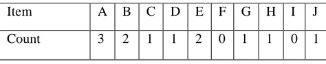
pattern alone are considered and recorded in the tables. Mining can be done in the data source as follows :I Start scanning the Item A B C D E F G H I J

Count 3 2 1 1 2 0 1 1 0 1

Item

Segment a b c d e f g h i j Horizo_ntal

count hi ISV1 3 2 1 1 2 0 1 1 0 1 9

ISV2 3 3 3 2 0 1 0 0 1 0 11

ISV3 2 2 2 1 1 1 0 0 1 1 8

Vertical

segments in the order of their priority i.e., descending order of hi. For each segment apply the following

1. Read a transaction t, when the segment is not empty 2. Consider frequent items alone (pattern)

3. Check for the pattern in Maximal Frequent Table

a. If Maximal Frequent Table is null, goto step 4.

b.If the new pattern is a subset of an already existing pattern then goto step 1.

c. If the new pattern is similar to an already existing pattern, then increment the count of the already existing pattern by one and goto step 1.

d. If the new pattern is a superset of an already existing pattern then increment the count of the existing pattern by one and goto step 4.

4. Check for the pattern in Maximal Frequent Candidate Table

a. If the incoming pattern is similar to an existing pattern then increment its count by one

b. If the incoming pattern is superset of an existing pattern then increment the count of its sub pattern by one and insert the new pattern into Maximal Frequent Candidate Table with its count initialized to 1.

c If the incoming pattern is a subset of an existing pattern then insert the new pattern into Maximal Frequent Candidate Table with its count initialized to the sum of the supports of its supersets in Maximal Frequent Candidate Table plus one. d If the incoming pattern is a new pattern, record the new pattern in the Maximal Frequent Candidate Table and initialize its count to one.

5. If any of the patterns in the Maximal Frequent Candidate Table has reached the minimum support threshold, move that pattern to Maximal Frequent Table. Simultaneously prune all its sub patterns from the Maximal Frequent Table.

Determine all the common frequent patterns from the patterns in Maximal Frequent Candidate Table and calculate its support which is equal to the sum of the support of its supersets in Maximal Frequent Candidate Table. Add it to the Maximal

Frequent Table when its support passes the minimum threshold.

Example:

For the data source given in Table 2 mining is done as follows Step 1:

After mining segment 2:

Maximal Frequent Table contains {abc :3}

Maximal frequent candidate table contains the items{abcd:2}

After mining segment 1:

Maximal Frequent Table contains the itemsets {abc : 4}

Maximal Frequent Candidate Table contains the items

{ade:1,abce:1,abcd:2} After mining segment 3:

Maximal frequent table contains the itemsets {abcd:3}

Maximal frequent candidate table contains the items { ade:1,abce:2 }

STEP II:

Common frequent patterns in maximal frequent table{ae:3} Maximal frequent table contains the itemsets { abcd:3, ae:3} Finally all the MFS are available in maximal frequent table Thus it is seen that the proposed technique generates the same MFS as those generated by the Pincer approach of (Lin and Kedem,2002).

V. PERFORMANCE EVALUATION

The experiment was conducted on a Pentium IV computer with a CPU clock rate of 2.8 GHz, 2 GB RAM running Windows Operating System. The data sources for the experiment were generated synthetically. Three data sources 10K, 50K, and 100K were generated to study theperformance of the proposed work. Table 5 shows the characteristics of each data source. The performance of the proposed approach has extensively been studied to confirm its effectiveness.

Table 8: Summary of sample data sources taken for performance study

Name |T| |I| |D|

Data source 1 Data source 2 Data source 3

10 10 10

3 3 3

10K 50K 100K

The MFS generated by the proposed technique has been found to be identical to the MFSgenerated by the Pincer Approach.

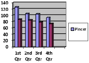
Tables 6, 7, and 8 simply compare the performance of the proposed technique with the Pincer technique

Figure 2 displays the diagrammatic representation of these results.

VI. CONCLUSIONS

While the problems considered in this paper are novel and important to the area of ad hoc data exploration and retrieval, we observe that our specific problem definition does have limitations. After all, a query log is only an approximate surrogate of real user preferences, and moreover, in some applications neither the database, nor the query log may be available for analysis; thus, we have to make assumptions about the nature of the competition as well as about the user preferences. Finally, in all these problems, our focus is on deciding what subset of attributes to retain of a product

REFERENCES

[1] D. Burdick, M. Calimlim, and J. Gehrke, (2001)“MAFIA: A Maximal Frequent Item Set Algorithm for Transactional Databases,” Proc. Int’l Conf. Data Eng. (ICDE), 2001.

[2] M.R. Garey and D.S. Johnson (1979), “Computers and Intractability: A Guide to the Theory of NP-Completeness”.

[3] W.H. Freeman, K. Gouda and M.J. Zaki, (2001) “Efficiently Mining

Maximal Frequent Itemsets,” Proc. Int’l Conf. Data Mining (ICDM), [4] J. Han, J. Pei, and Y. Yin, (2000) “Mining Frequent Patterns without

Candidate Generation,” Proc. SIGMOD Conf., pp. 1-12,. J. Han, J. Wang, Y. Lu, and P. Tzvetkov, (2002) “Mining Top-k Frequent Closed Patterns

without Minimum Support,” Proc. Int’l Conf. Data Mining (ICDM),. [5] M.D. Morse, J.M. Patel, and H.V. Jagadish, (2007) “Efficient Skyline

Computation over Low-Cardinality Domains,” Proc. Int’l Conf.Very Large Data Bases (VLDB),.

[6] M. Miah, G. Das, V. Hristidis, and H. Mannila, (2008) “Standing Out in a

Crowd: Selecting Attributes for Maximum Visibility,” Proc. Int’l Conf. Data Eng. (ICDE), pp. 356-365, 2008.

AUTHORS

First Author – Murlidher Mourya, M.Tech,Vardhaman College of Engineering, [email protected].