R E S E A R C H
Open Access
A generalized gradient projection method
based on a new working set for minimax
optimization problems with inequality
constraints
Guodong Ma
1*, Yufeng Zhang
2and Meixing Liu
1*Correspondence: [email protected] 1School of Mathematics and Statistics, Guangxi Colleges and Universities Key Laboratory of Complex System Optimization and Big Data Processing, Yulin Normal University, Yulin, China Full list of author information is available at the end of the article
Abstract
Combining the techniques of the working set identification and generalized gradient projection, we present a new generalized gradient projection algorithm for minimax optimization problems with inequality constraints. In this paper, we propose a new optimal identification function, from which we provide a new working set. At each iteration, the improved search direction is generated by only one generalized gradient projection explicit formula, which is simple and could reduce the computational cost. Under some mild assumptions, the algorithm possesses the global and strong convergence. Finally, the numerical results show that the proposed algorithm is promising.
MSC: 90C30; 49K35; 65K05
Keywords: minimax optimization problems; inequality constraints; generalized gradient projection method; global and strong convergence
1 Introduction
Minimax problem is an important class of nonsmooth optimization, since it has a broad application background. Numerous models in optimal control [, ], engineering prob-lem [], portfolio optimization [] and many other situations [] can be formulated as the following minimax optimization problems with inequality constraints:
minF(x), s.t.fj(x)≤, j∈J, ()
whereF(x) =max{fj(x),j∈I}withI={, , . . . ,m},j∈J={l+,l+, . . . ,l+m},fj(x) :Rn→R
(j∈I∪J) are continuously differentiable functions. The objective functionF(x) is not necessarily differentiable, even when allfj(x),j∈ {I∪J}are differentiable. Obviously, the
non-differentiablity of the objective functionF(x) is a main challenge for solving minimax problem, as the classical smooth methods cannot be applied directly. Over the past few decades, the minimax problem has attracted more and more researchers’ attention and many algorithms have been developed, which can be grouped into three classes in general.
The first class of algorithms views the problem () as the constrained nonsmooth opti-mization problem, which can be solved directly by several classical nonsmooth methods, such as subgradient methods, bundle methods, and cutting plane methods, Refs. [–]. The algorithms in [–] have a shortcoming that it is difficult to improve the numerical results. However, we have observed in [] that a feasible descent bundle method for solv-ing inequality constrained minimax problems is proposed, by ussolv-ing the subgradients of functions, the idea of bundle method and the technique of partial cutting planes model, to generate the new cutting plane and aggregate the subgradients in the bundle, so the difficulty of numerical calculation and storage is overcome.
The second one is the entropy function method [–]. First, it transforms the objective function minimax problem into a smooth function with parameters. Then the objective function is approximated by a parametric and smooth function. For example, the para-metric and smooth function with the parameterp
Fp(x) =
pln
l
i=
exppfi(x)
.
Since ≤Fp(x) –F(x)≤plnl, sop→ ∞,Fp(x)→F(x).
Due to the particular structure of the objective function, the third approach is that the problem () can be transformed into the following equivalent smooth constrained nonlin-ear programming by introducing an artificial variablez:
min
(x,z)∈Rn+z, s.t.fi(x) –z≤, i∈I; fj(x)≤, j∈J.
Then, we can solve the above inequality constrained optimization by some well-established methods, such as the sequential quadratic programming type (SQP) methods [–], the sequential quadratically constrained quadratic programming type (SQCQP) methods [, ], the trust-region strategy [, ] and the interior-point method []. In [], a SQP algorithm is proposed that incorporates the particular case of minimax problems, the global and local convergence is ensured. In order to improve the conver-gence properties and numerical performance, Jian and Zhuet al. developed improved SQP methods established in [, ] for solving unconstrained or constrained minimax prob-lems, by means of solving one quadratic programming an improved direction is yielded and a second-order correction direction can also be at hand via one system of linear equa-tions. Under mild conditions, we can ensure global and superlinear convergence. Jianet al. [] developed the norm-Relaxed SQP method based on active set identification and new line search for constrained minimax problems, which the master direction and high-order correction direction are computed by solving a new type of norm-relaxed quadratic pro-gramming subproblem and a system of linear equations, respectively. Moreover, the step size is yielded by a new line search which combines the method of strongly sub-feasible direction with the penalty method.
al. [] also proposed the simple sequential quadratically constrained quadratic program-ming algorithm for smooth constrained optimization. Unlike the previous work, at each iteration, the main search direction is obtained by solving only one subprogram which is composed of a convex quadratic objective function and simple quadratic inequality con-straints without the second derivatives of the constrained functions.
Although the SQP and SQCQP methods can effectively solve the minimax problem, this transformation may ignore the unique nature of the minimax problem and then increase the number of constraint functions. Moreover, these methods require the solution of one or two QP (QCQP) subproblems at each iteration, especially, some subproblems may be complex for the large-scale problems. In general, there are many cases where the sub-problems cannot be solved easily, which will increase the amount of computations largely. Hence, (generalized) gradient projection method (GGPM) based on the Rosen gradient projection method [] has been developed for solving inequality constrained optimiza-tion problems. The GGPM method has good properties that the search direcoptimiza-tion is only a gradient projection explicit formula and it has nice convergence and numerical results for middle-small-scale problems. These good natures cause widespread concern of many scholars [–]. In [], Chapter II, there are more systematic and detailed study about generalized gradient projection algorithm for inequality constrained smooth optimiza-tion.
It is well established in the literature that, when the number of constraints is very large, the active set identification technique can improve the local convergence behavior and decrease the computation cost of the algorithms of nonlinear programming and mini-max problems. An earlier study of the active set identification technique can be found in []. Many satisfactory results on the general nonlinear case were studied,e.g., [, ]. Facchineiet al. [] described a technique based on the algebraic representation of the constraint set, which identifies active constraints in a neighborhood of a solution. The ex-tension to constrained minimax problems was also first presented in [] without strict complementarity and linear independence. Moreover, the identification technique of ac-tive constraints for constrained minimax problems can be more suitable for infeasible al-gorithms, such as the strongly sub-feasible direction method and the penalty function method.
Despite GGPM’s importance and usefulness, there are no GGPM type method that are applied to solve minimax problems with inequality constraints. The aim of this paper is to propose such an algorithm, analyze its convergence properties, and report its numeri-cal performance. Motivated by [, ], in this paper, we propose a generalized gradient projection algorithm directly onRnwith a new working set for the problem (). The char-acteristics of our proposed algorithm can be summarized as follows:
. We propose a new optimal identification function for the stationary point, from which we provide a new working set.
. The search direction is generated by only one generalized gradient projection explicit formula, which is simple and could reduce the computational cost. . Under some mild assumptions, the algorithm possesses the global and strong
convergence.
2 Description of algorithm
In this section, for the sake of simplicity, we introduce and use the following notations for the problem () in this paper:
X:=x∈Rn:fj(x)≤,j∈J
, ()
I(x) :=i∈I:fi(x) =F(x)
, J(x) :=j∈J:fj(x) =
. ()
According to the analysis of other projection algorithms, we need the following linear independence assumption.
Assumption A The functionsfj(x) (j∈I∪J) are all first order continuously
differen-tiable, and there exists an index lx∈I(x) for each x∈Xsuch that the gradient vectors
{∇fi(x) –∇flx(x),i∈I(x)\{lx};∇fj(x),j∈J(x)}are linearly independent.
Remark We can easily find that Assumption A is equivalent to Assumption A-:
Assumption A- The vectors{∇fi(x) –∇ft(x),i∈I(x)\{t};∇fj(x),j∈J(x)}are linearly
in-dependent for arbitrarilyt∈I(x).
For a given pointxkand the parameterε≥, we use the following approximate active
set in this paper:
⎧ ⎨ ⎩
Ik={i∈I: –˜k≤fi(xk) –F(xk)≤},
Jk={j∈J: –˜k≤fj(xk)≤},
()
where˜kis taken by
˜
=ε, ˜k=min{ε,k–}, k≥, () k–≥ is the identification function corresponding to the last iteration pointxk–and it
can be calculated by (). At each iteration, onlykneed to be computed, sincek–has
already been calculated at the previous iteration, so the total computing capacity is not increase at each iteration.
For the current iteration pointxk, for convenience of statement, we define
Fk:=Fxk, fk i :=fi
xk, gik:=∇fi
xk, i∈I∪J, lk∈I
xk, Ik:=Ik\{lk}, Lk:=Ik∪Jk:= (Ik∪Jk)\{lk},
wherelk∈I(xk). In theory, the indexlkcan be any component of the active setI(xk) of
Algorithm A, and all the theoretical analyses are the same. But we setlk=lxk=:min{i: i∈I(xk)}for convenience. We can easily find thatI(xk)⊆I
k,J(xk)⊆Jk. Therefore, for the
feasible point xk of the problem (), its stationary point (optimality conditions) can be
described as
⎧ ⎨ ⎩
i∈Ikλ
k igik+
j∈Jkλ
k jgjk= ,
i∈Ikλ
k i = ,
λik≥,λki(fik–Fk) = ,i∈Ik;λkj ≥,λkjfjk= ,j∈Jk.
The foregoing conditions can be rewritten in the following equivalent form: ⎧ ⎪ ⎪ ⎪ ⎨ ⎪ ⎪ ⎪ ⎩
i∈Ikλki(gik–glkk) +
j∈Jkλ
k
jgjk= –glkk,
λik≥,λki(fik–Fk) = ,i∈I
k;λkj ≥,λjkfjk= ,j∈Jk,
λkl
k= –
i∈Ikλki ≥.
()
We define a generalized gradient projection matrix to test whether the current iteration pointxksatisfies ()
Pk:=En–NkQk, ()
whereEnis annth-order identity matrix.
Nk:=
gik–gklk,i∈Ik;gjk,j∈Jk
, Qk:=
NkTNk+Dk
–
NkT, ()
Dk:=diag
Dkj,j∈Lk
, Dkj :=
⎧ ⎨ ⎩
(Fk–fjk)p, j∈Ik; (–fjk)p, j∈J
k.
()
Suppose that (xk,λk
Lk) is a stationary point pair, from (), it is not difficult to get NkTNkλkLk= –N
T
kglkk, Dkλ
k
Lk= , λ
k Lk≥. These further imply that
NkTNk+Dk
λkL
k= –N
T
kgklk, λ
k
Lk= –Qkg
k
lk, ()
Pkglkk= , λ
k
lk≥, D
k
jλkj = , λkj ≥, j∈Lk. ()
Based on the above analysis, we introduce the following optimal identification function for the stationary point:
ρk:=Pkglkk
+ωk+ω¯k, ()
where
ωk:=
j∈Lk
max–μkj,μkjDkj, ω¯k:=max
–μkl
k,
, ()
μkL
k:= –Qkg
k lk, μ
k lk:= –
i∈Ik
μki. ()
Before describing our algorithm, one has the following lemma.
Lemma Suppose that AssumptionAholds.Then
(i) the matrixNT
kNk+Dkis nonsingular and positive definite.Supposexk→x∗,
Nk→N∗,Dk→D∗,then the matrixN∗TN∗+D∗is also nonsingular and positive
(ii) NT
kPk=DkQk,NkTQTk =E|Lk|–Dk(N
T
kNk+Dk)–;
(iii) (glk k)
TP
kglkk=Pkglkk+
j∈Lk(μ
k j)Dkj;
(iv) ρk= if and only ifxkis a stationary point of the problem().
Proof Under Assumption A, it is shown that the matrixNT
kNk+Dk is nonsingular by
[], Theorem ... Then, we can prove that the matrixNT
∗N∗+D∗is also definite similar
to [], Lemma ... The conclusions (ii) and (iii) can obtained similar to [], Theo-rem ... Next, we prove the conclusion (iv) in detail below.
(iv) Ifρk= , combining the equations (), (), and (), we obtain
=Pkglkk=g
k
lk–NkQkg
k lk=g
k lk+Nkμ
k Lk. We havemax{–μk
j,μkjDj}= byωk= , which follows byμkj ≥,μkjDkj = ,∀j∈Lkand it
is not difficult to getμkl
k ≥ byω¯k= . So we have
⎧ ⎨ ⎩
i∈Ikμ
k igik+
j∈Jkμ
k jgjk= ,
i∈Ikμ
k i = ,
μki ≥,μki(fk
i –Fk) = ,i∈Ik;μkj ≥,μkjfjk= ,j∈Jk.
Therefore, xk is a stationary point of the problem () with the multiplier
(μkI
k∪Jk, (I∪J)\(Ik∪Jk)).
Conversely, ifxkis a stationary point of the problem () with the multiplier vectorλk,
then from the ()-() one knows thatμkL
k=λ
k
Lk, andρk= .
The above results show that the current iteration pointxk is a stationary point of the problem () if and only ifρk= , that is,ρk is optimal identification function. In case of
ρk> , together withIkandJk, we compute the search direction, which is motivated by
the generalized gradient projection technique in [], Chapter II, and []
dk=ρkξ–Pkgklk+Q
T kvkLk
–kQTkek, ()
where the parameterξ> ,ek= (, , . . . , )T∈R|Lk|,
k=
ρk+ξ
+μkL
k
, ()
the vectorvkLk= (vkj,j∈Lk) with
vkj =
⎧ ⎨ ⎩ ¯
ωk– , ifμkj < ,j∈Ik;
¯
ωk+Dkj, ifμkj ≥,j∈Ik,
vkj =
⎧ ⎨ ⎩
–, ifμk
j < ,j∈Jk;
Dkj, ifμkj ≥,j∈Jk.
()
The following lemma further describes the important characteristics of the search direc-tion, which is feasible and descent.
Lemma Suppose that AssumptionAholds.Then
(i) (glk k)
Tdk≤–ρξ
kω¯k–k;
(ii) (gjk)Tdk≤–
(iii) F(xk;dk)≤–
k,whereF(xk;dk)is the directional derivative ofF(x)at the pointxk
along the directiondk.
Proof (i) First, by (), together with Lemma (iii), (), () and (), we obtain
glkkTdk=ρkξ–glkkTPkglkk+
Qkglkk
T
vkLk–k
Qkglkk
T
ek =ρkξ
–Pkgklk
–
j∈Lk
μkjDkj –μkL
k
T
vkL k
+k
μkL
k
T
ek
≤ρkξ
–Pkglkk
–
μki<,i∈Ik
μki(ω¯k– ) –
μki≥,i∈Ik
μkiω¯k+Dki
–
μkj<,j∈Jk
–μkj– μkj≥,j∈Jk
μkjDkj
+k
μkL
k
T
ek
=ρkξ
–Pkgklk
–
μkj<,j∈Lk
–μkj– μkj≥,j∈Lk
μkjDkj –ω¯k
i∈Ik
μki
+k
μkL
k
T
ek
=ρkξ
–Pkgklk
–ωk–ω¯k
i∈Ik
μki
+k
μkL
k
T
ek.
In addition, based on the definition of μkl
k, it immediately follows ω¯k
i∈Ikμki =ω¯k+
¯
ωk(–μklk). Ifμ
k
lk ≥, we haveω¯k= ,ω¯k(–μ
k
lk) = =ω¯
k. On the other handμklk< , then
¯
ωk= –μklk,ω¯k(–μ
k lk) =ω¯
k. Thus,ω¯k
i∈Ikμki =ω¯k+ω¯kis always true. We have from ()
and ()
glkkTdk≤ρkξ–Pkglkk
–ωk–ω¯k–ω¯k
+k
μkL
k
T
ek =ρkξ(–ρk–ω¯k) +k
μkL
k
T
ek
≤–ρkξω¯k–ρk+ξ+kμkLk
= –ρkξω¯k–k. ()
(ii) From Lemma (ii) and (), we obtain
NkTdk=ρξk–NkTPkglkk+N
T kQTkvkLk
–kNkTQTkek
=ρξk–DkQkglkk+v
k Lk–Dk
NkTNk+Dk
–
vkLk –k
E|Lk|–Dk
NkTNk+Dk
–
ek. ()
Then we discuss the following two cases, respectively. Case .Fori∈(I(xk)\{l
k})⊆Ik, it follows thatDjk= . From (), we have (gik–glkk)
Tdk=
ρkξvki –k. Then, combined () with conclusion (i), we have
Case .Forj∈J(xk)⊆J
k,Dkj = holds. It follows from () and () that
gjkTdk=ρkξvkj –k≤–k.
By summarizing the above discussion, the conclusion (ii) holds. (iii) SinceF(xk;dk) =max{(gk
i)Tdk,i∈I(xk)}, we haveF(xk;dk)≤–kfrom the
conclu-sions (i) and (ii).
Based on the improved direction dk defined by () and analysed above, we are now ready to describe the steps of our algorithm as follows.
Algorithm A Step .Choose an initial feasible pointx∈Xand parameters:α,β∈(, ), ε> ,p≥,ξ> . Letk:= .
Step .For the current iteration pointxk, generate the working setI
k,Jkby () and (),
calculate the projection matrixPk, the optimal identification function valuesρkandk
by (), ()-() and (). Ifρk= , thenxkis a stationary point of the problem (), stop.
Otherwise, go to Step .
Step .Obtain the search directiondkby ()-().
Step .Compute the step sizetk, which is the maximumtof the sequence{,β,β, . . .}
satisfying
Fxk+tdk≤Fk–αtk, ()
fj
xk+tdk≤, j∈J. ()
Step .Letxk+=xk+t
kdk,k:=k+ , and go back to Step .
Remark The inequality () is equivalent tofi(xk+tdk)≤Fk–αtk,i∈I.
Note that Lemma , we getF(xk;dk)≤–
k< and (gkj)Tdk≤–k,∀j∈J(xk), so it is easy
to know that () and () hold fort> small enough, then Algorithm A is well defined.
3 Convergence analysis
In this section, we will analyze the global and strong convergence of Algorithm A. If Al-gorithm A stops atxkin a finite number of iterations, thenρ
k= . From Lemma (iv), we
know thatxkis a stationary point of the problem (). Next, we assume that Algorithm A
yields an infinite iteration sequence{xk}of points, and prove that any accumulation point
x∗of{xk}is a stationary point for the problem () under some mild conditions including
the following assumption.
Assumption A The sequence{xk}generated by Algorithm A is bounded. Lemma Suppose that AssumptionsAandAhold.Then
(i) there exists a positive numbercsuch thatdk ≤cρξ
k;
(ii) limk→∞xk+–xk= .
Proof (i) Because of Assumption A and Lemma (i), it is easy to get the total sequences
{Pk}∞k=and{Qk}∞k= of matrices are bounded. Furthermore, from () and (), we know
that{μkL
k}and{v
k
Lk}are bounded. This implies thatd
k ≤cρξ
(ii) In view of{F(xk)}is decreasing and bounded, solim
k→∞F(xk) =F(x∗). Then,
com-bining () with the definition ofk, one haslimk→∞tkρ+
ξ
k = . Taking into account the
parameterξ> , it follows that
lim
k→∞
xk+–xk= lim
k→∞tk
dk≤ lim
k→∞ctkρ
ξ
k=cklim→∞
tkρ+k ξ
ξ tk
+ξ = .
Based on the lemma above, we can present the global convergence of our algorithm.
Theorem Suppose that AssumptionsAandAhold.Then AlgorithmAgenerates an infinite sequence{xk}of points such that each accumulation x∗of{xk}is a stationary point
of the problem().
Proof If the infinite iteration index set K satisfies limk∈Kxk = x∗, it follows that
limk∈Kxk–=x∗from Lemma (ii). Noting thatI
k,Jkandlkare finite, we suppose∀k∈K
(choosing a subsequence ofKwhen necessary) satisfies
Ik≡I∗, Jk≡J∗, lk≡l∗, Ik≡I∗:={I∗}\l∗, Lk≡L∗:=I∗∪J∗, ()
Ik–≡ ¯I∗, Jk–≡ ¯J∗, lk–≡ ¯l∗,
Ik–≡ ¯I∗:={¯I∗}\¯l∗, Lk–≡ ¯L∗:=I¯∗∪ ¯J∗.
()
Define
D∗j =
⎧ ⎨ ⎩
(F(x∗) –fj(x∗))p, j∈I∗\{l∗};
(–fj(x∗))p, j∈J∗,
D∗=diagD∗j,j∈L∗
, ()
N∗=∇fi
x∗–∇fl∗
x∗,i∈I∗;∇fj
x∗,j∈J∗, P∗=En–N∗Q∗, ()
Q∗=N∗TN∗+D∗–N∗T,μ∗L∗=
μ∗j,j∈L∗= –Q∗∇fl∗
x∗, ()
ω∗=
j∈L∗
max–μ∗j,μ∗jD∗j, μ∗l∗= –
i∈I∗
μ∗i, ω¯∗=max–μ∗l∗, , ()
ρ∗=P∗∇fl∗
x∗+ω∗+ω¯∗, ∗= ρ +ξ
∗
+μ∗L∗
. ()
The above definitions are well defined by Lemma (i). Similarly, forx∗,¯I∗,¯J∗and¯l∗, we
defineρ¯∗ and¯∗. In addition, the matrixNT
∗N∗+D∗is positive definite by Lemma (i). Therefore, the sequences{vk}
Kand{dk}K are bounded. Then, assume by contradiction thatx∗is not the stationary point of the problem (), we can easily get∗> and¯∗> similar to the analysis of Lemma (iv). Then, we have
k≥.∗, k–→ ¯K ∗:= ¯ ρ∗
+ ¯μ∗¯
L∗ > ,
˜
k=min{ε,k–}→K ∼∗ :=min{ε,¯∗}> .
A. The step size sequence {tk}k∈K is always bounded away from zero, that is, ¯t:=
inf{tk,k∈K}> . We only need to show the inequalities () and () hold fork∈Klarge
enough andt> sufficiently small.
A. Fori∈I, in this case, we havei∈/I(x∗) andi∈I(x∗) as two cases.
A. Casei∈/I(x∗), that isfi(x∗) <F(x∗). Taking into account the differentiability offi(x)
and the boundedness of{dk}Kand using Taylor expansion, we have fi
xk+tdk–Fk+αtk=fik+t
gikTdk+o(t) –Fk+αtk
=fik–Fk+O(t)
≤.fi
x∗–Fx∗+O(t)
≤.
A. Casei∈I(x∗), that is,fi(x∗) =F(x∗). Note thatxk→x∗and∼∗ > , by () and (),
we know thatI(x∗)⊆Ikalways holds fork∈Klarge enough. Hence,i∈Ik. In this case,
we also have two cases, which arei=l∗ andi=l∗. Therefore, we discuss the two cases, respectively.
Assumei=l∗, it follows by Lemma (i) that
glk∗Tdk≤–ρkξω¯k–k≤–k. ()
Assumei=l∗,Dki = (Fk–fik)p→K (F(x∗) –fi(x∗))p= . From Lemma (i), we have (NkTNk+
Dk)–→(N∗TN∗+D∗)–. Together with () we conclude that
gik–glk k
T
dk=ρkξvki–k+O
Dki.
In view of (),vki ≤ ¯ωk+O(Dki) holds. Combining () withk→∗> , we have
gikTdk≤ρkξω¯k+
glk k
T
dk–k+O
Dki≤–k+O
Dki≤–k. ()
Thus, fori∈I(x∗), from () and (), using Taylor expansion, we obtain
fi
xk+tdk–Fk+αtk≤fik+t
gikTdk+o(t) –fik+αtk
≤–( –α)tk+o(t)
≤–.t( –α)∗+o(t) ≤.
According to the analysis of the above A and A, it is sufficient to show that the in-equality () is always satisfied fork∈Klarge enough andt> sufficiently small.
A. Forj∈J, there are alsoj∈/J(x∗) andj∈J(x∗) two cases.
A. Casej∈/ J(x∗), it follows thatfj(x∗) < . Taking into account the boundedness of
{dk}
Kand using Taylor expansion, we have
fj
xk+tdk=fjk+O(t)≤.fj
A. Casej∈J(x∗), that is,fj(x∗) = .j∈Jk follows in a similar analysis to A, and we
haveDkj = (–fjk)p→K . By recalling (), (gk
j)Tdk=ρ
ξ
kvkj –k+O(Dkj). Then using Taylor
expansion and (), we get
fj
xk+tdk=fjk+tgjkTdk+o(t)
≤fjk–tk+tO
Dkj+o(t)
≤–.t∗+o(t)
≤.
Thus, inequality () always holds fork∈K large enough and t> sufficiently small. Hence,t¯:=inf{tk,k∈K}> holds.
B. Export contradiction by usingtk≥ ¯t> (k∈K). In view of (), it is easy to know
that the sequence {Fk} is monotone nonincreasing. Since lim
k∈KFk=F(x∗), it implies
limk→∞Fk=F(x∗). This, together with () andtk≥ ¯t,k≥.∗, we have
Fx∗=lim
k∈KF
k+≤lim
k∈K
Fk–αtkk
≤lim
k∈K
Fk– .α¯t∗=Fx∗– .α¯t∗,
which contradicts¯t> and∗> . Therefore,x∗is a stationary point for the problem (),
and the whole proof is completed.
Subsequently, we further show that Algorithm A has the property of strong convergence.
Theorem Suppose that AssumptionsAandAhold.If the sequence{xk}of points
gen-erated by AlgorithmApossesses an isolated accumulation point x∗,thenlimk→∞xk=x∗,
that is,AlgorithmAis strongly convergent.
Proof Since the sequence{xk}of points generated by Algorithm A possesses an isolated
accumulation point, together withlimk→∞xk+–xk= (Lemma (ii)) and [],
Corol-lary .., we immediately havelimk→∞xk=x∗. Finally, bylimk→∞xk=x∗and Theorem ,
it follows thatx∗is the stationary point of the problem ().
4 Numerical experiments
Table 1 Numerical results of Algorithm A
Prob. n/l/m x0 NI NF NC F(x∗) T (s)
P1 2/3/2 (1, 2.4)T 15 115 33 1.952225 0.03
P2 2/3/2 (0, 1)T 31 44 63 2.000009 0.01
P3 4/4/3 (0, 0.9, 0.9, –1.5)T 28 143 89 –43.999992 0.01
P4 2/6/2 (1, 2.4)T 18 379 37 0.616433 0.02
P5 50/2/48 (2,. . ., 2)T 85 551 4299 –69.296460 0.27
P6 50/2/48 (0.5,. . ., 0.5)T 150 6061 17026 –56.502976 0.79
P7 100/2/98 (0.5,. . ., 0.5)T 22 160 2157 0.000006 0.13
P8 100/100/98 (1,. . ., 1)T 98 691 9605 0.500009 1.22
P9 200/3/199 (0.5,. . ., 0.5)T 102 1087 22502 398.000010 2.72
P10 200/2/198 (1,. . ., 1)T 150 456 29723 111.701918 3.92
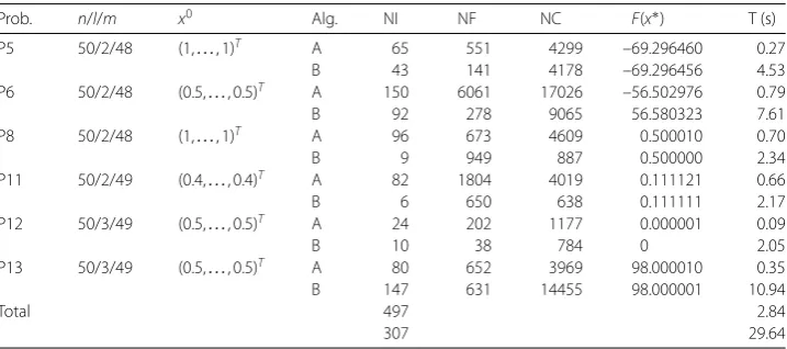
Table 2 Numerical comparisons for Algorithms A and B
Prob. n/l/m x0 Alg. NI NF NC F(x∗) T (s)
P5 50/2/48 (1,. . ., 1)T A 65 551 4299 –69.296460 0.27
B 43 141 4178 –69.296456 4.53
P6 50/2/48 (0.5,. . ., 0.5)T A 150 6061 17026 –56.502976 0.79
B 92 278 9065 56.580323 7.61
P8 50/2/48 (1,. . ., 1)T A 96 673 4609 0.500010 0.70
B 9 949 887 0.500000 2.34
P11 50/2/49 (0.4,. . ., 0.4)T A 82 1804 4019 0.111121 0.66
B 6 650 638 0.111111 2.17
P12 50/3/49 (0.5,. . ., 0.5)T A 24 202 1177 0.000001 0.09
B 10 38 784 0 2.05
P13 50/3/49 (0.5,. . ., 0.5)T A 80 652 3969 98.000010 0.35
B 147 631 14455 98.000001 10.94
Total 497 2.84
307 29.64
Algorithm A is coded in MATLAB Rb, and on a PC computer with Windows , Intel(R) Pentium(R) CPU . GHz. During the numerical experiments, we set parameters
α= .,β= .,ε= ,p= ,ξ= .. Execution is terminated ifρk< –or NI≥.
The numerical results are listed in Tables and . The following notations are used: ‘Prob.’: the test problem number; ‘n’: the dimensions of the variablex; ‘l‘: number of all component objective functions; ‘m’: number of constraint functions; ‘x’: initial feasible
point; ‘Alg.’: algorithm; ‘A and B’: the algorithms of this paper and [], respectively. ‘NI’: number of iterations; ‘NF’: number of all component functions evaluations in the objective; ‘NC’: number of constraints evaluations; ‘T’: CPU time (in seconds); ‘-’: the corresponding datum are not reported; ‘F(x∗)’: final objective value.
From Table , we see that Algorithm A can generate approximately optimal solution for all the test problems. The search direction is generated by the generalized gradient projection explicit formula, and a new working set is used, which can reduce the scale of the generalized gradient projection, so the proposed Algorithm A is efficient.
In Table , we compare our Algorithm A with Algorithm B, and all the numerical re-sults are tested by a same PC computer. The performance of the two algorithms is similar in terms of the approximate optimal objective value at the final iteration point, although the number of all component functions evaluations in the objective and constraints eval-uations is few for Algorithm B, our proposed algorithm performs much better than Algo-rithm B relative to the cost of CPU running times.
[image:12.595.119.478.247.406.2]5 Conclusions
Although the generalized gradient projection algorithms have good theoretical conver-gence and effectiveness in practice, their applications to minimax problems have not yet been investigated. In this paper, we present a new generalized gradient projection algo-rithm for minimax optimization problems with inequality constraints.
The main conclusions of this work:
() A new approximation working set is presented.
() Using the technique of generalized gradient projection, we construct a generalized gradient projection feasible decent direction.
() Under mild assumptions, the algorithm is global and strong convergent.
() Some preliminary numerical results show that the proposed algorithm performs efficiently.
6 Results and discussion
In this work, a new generalized gradient projection algorithm for minimax optimization problems with inequality constraints is presented. As further work, we think the ideas can be extended to minimax optimization problems with equality and inequality constraints and other optimization problems.
Competing interests
The authors declare that they have no competing interests.
Authors’ contributions
GDM carried out the idea of this paper, the description of Algorithm A and drafted the manuscript. YFZ carried out the convergence the analysis of Algorithm A. MXL participated in the numerical experiments and helped to draft the manuscript. All authors read and approved the final manuscript.
Author details
1School of Mathematics and Statistics, Guangxi Colleges and Universities Key Laboratory of Complex System Optimization and Big Data Processing, Yulin Normal University, Yulin, China. 2College of Mathematics and Information Science, Guangxi University, Nanning, China.
Acknowledgements
Project supported by the Natural Science Foundation of China (No. 11271086), the Natural Science Foundation of Guangxi Province (No. 2015GXNSFBA139001) and the Science Foundation of Guangxi Education Department (No. KY2015YB242) as well as the Doctoral Scientific Research Foundation (No. G20150010).
Received: 20 December 2016 Accepted: 12 February 2017 References
1. Baums, A: Minimax method in optimizing energy consumption in real-time embedded systems. Autom. Control Comput. Sci.43, 57-62 (2009)
2. Li, YP, Huang, GH: Inexact minimax regret integer programming for long-term planning of municipal solid waste management - part A, methodology development. Environ. Eng. Sci.26, 209-218 (2009)
3. Michelot, C, Plastria, F: An extended multifacility minimax location problem revisited. Ann. Oper. Res.111, 167-179 (2002)
4. Cai, XQ, Teo, KL, Yang, XQ, Zhou, XY: Portfolio optimization under a minimax rule. Manag. Sci.46, 957-972 (2000) 5. Khan, MA: Second-order duality for nondifferentiable minimax fractional programming problems with generalized
convexity. J. Inequal. Appl.2003, 500 (2013)
6. Gaudioso, M, Monaco, MF: A bundle type approach to the unconstrained minimization of convex nonsmooth functions. Math. Program.23, 216-226 (1982)
7. Polak, E, Mayne, DQ, Higgins, JE: Superlinearly convergent algorithm for min-max problems. J. Optim. Theory Appl.
69, 407-439 (1991)
8. Gaudioso, M, Giallombardo, G, Miglionico, G: An incremental method for solving convex finite min-max problems. Math. Oper. Res.31, 173-187 (2006)
9. Jian, JB, Tang, CM, Tang, F: A feasible descent bundle method for inequality constrained minimax problems. Sci. Sin., Math.45, 2001-2024 (2015) (in Chinese)
10. Xu, S: Smoothing method for minimax problems. Comput. Optim. Appl.20, 267-279 (2001)
12. Polak, E, Womersley, RS, Yin, HX: An algorithm based on active sets and smoothing for discretized semi-infinite minimax problems. J. Optim. Theory Appl.138, 311-328 (2008)
13. Xiao, Y, Yu, B: A truncated aggregate smoothing Newton method for minimax problems. Appl. Math. Comput.216, 1868-1879 (2010)
14. Zhou, JL, Tits, AL: An SQP algorithm for finely discretized continuous minimax problems and other minimax problems with many objective functions. SIAM J. Optim.6, 461-487 (1996)
15. Zhu, ZB, Cai, X, Jian, JB: An improved SQP algorithm for solving minimax problems. Appl. Math. Lett.22, 464-469 (2009)
16. Jian, JB, Zhang, XL, Quan, R, Ma, Q: Generalized monotone line search SQP algorithmfor constrained minimax problems. Optimization58, 101-131 (2009)
17. Jian, JB, Hu, QJ, Tang, CM: Superlinearly convergent norm-relaxed SQP method based on active set identification and new line search for constrained minimax problems. J. Optim. Theory Appl.163, 859-883 (2014)
18. Jian, JB, Chao, MT: A sequential quadratically constrained quadratic programming method for unconstrained minimax problems. J. Math. Anal. Appl.362, 34-45 (2010)
19. Jian, JB, Mo, XD, Qiu, LJ, Yang, SM, Wang, FS: Simple sequential quadratically constrained quadratic programming feasible algorithm with active identification sets for constrained minimax problems. J. Optim. Theory Appl.160, 158-188 (2014)
20. Wang, FS, Wang, CL: An adaptive nonmonotone trust-region method with curvilinear search for minimax problem. Appl. Math. Comput.219, 8033-8041 (2013)
21. Ye, F, Liu, HW, Zhou, SS, Liu, SY: A smoothing trust-region Newton-CG method for minimax problem. Appl. Math. Comput.199, 581-589 (2008)
22. Obasanjo, E, Tzallas-Regas, G, Rustem, B: An interior-point algorithm for nonlinear minimax problems. J. Optim. Theory Appl.144, 291-318 (2010)
23. Rosen, JB: The gradient projection method for nonlinear programming, part I. Linear constraints. J. Soc. Ind. Appl. Math.8, 181-217 (1960)
24. Du, DZ, Wu, F, Zhang, XS: On Rosen’s gradient projection methods. Ann. Oper. Res.24, 9-28 (1990)
25. Jian, JB: Fast Algorithms for Smooth Cconstrained Optimization - Theoretical Analysis and Numerical Experiments. Science Press, Beijing (2010) (in Chinese)
26. Ma, GD, Jian, JB: Anε-generalized gradient projection method for nonlinear minimax problems. Nonlinear Dyn.75, 693-700 (2014)
27. Burke, JV, More, JJ: On the identification of active constraints. SIAM J. Numer. Anal.25, 1197-1211 (1988)
28. Facchinei, F, Fischer, A, Kanzow, C: On the accurate identification of active constraints. SIAM J. Optim.9, 14-32 (1998) 29. Oberlin, C, Wright, SJ: Active set identification in nonlinear programming. SIAM J. Optim.17, 577-605 (2006) 30. Han, DL, Jian, JB, Li, J: On the accurate identification of active set for constrained minimax problems. Nonlinear Anal.
74, 3022-3032 (2011)