Generalized Maximum Entropy estimation of discrete sequential move games of perfect information

(1)

Munich Personal RePEc Archive

Generalized Maximum Entropy

estimation of discrete sequential move

games of perfect information

Wang, Yafeng and Graham, Brett

The Wang Yanan Institute for Studies in Economics (WISE)

20 December 2009

(2)

Generalized Maximum Entropy Estimation of Discrete

Sequential Move Games of Perfect Information

∗

Yafeng Wang

and

Brett Graham

†

Wang Yanan Institute for Studies in Economics (WISE)

Xiamen University

December 7, 2010

Abstract

We propose a data-constrained generalized maximum entropy estimator for discrete sequential move games of perfect information. Unlike most other work on the estimation of complete information games, the method we proposed is data constrained and requires no simulation or assumptions about the distribution of random preference shocks. We formulate the GME estimation as a (convex) mixed-integer nonlinear optimization prob-lem which can be easily impprob-lemented on optimization software with high-level interfaces such as GAMS. The model is identified with only weak scale and location normalizations. Monte Carlo evidence demonstrates that the estimator can perform well in moderately size samples. As an application we study the location choice of German siblings using the German Ageing Survey.

Keywords: Game-Theoretic Econometric Models, Sequential-Move Game,

General-ized Maximum Entropy, Mixed-Integer Nonlinear Programming.

JEL Classification Numbers: C01, C13, C35, C51, C72.

∗_{First version: Dec. 2009.}

(3)

1 Introduction

This paper focuses on the estimation of discrete sequential-move games of complete

in-formation. The estimation of complete information sequential-move games have received

less attention than their incomplete information counterparts 1

. since they involve

mul-tidimensional integrals which incorporates a higher degree of computational complexity.

Recently, Bajari, Hong, and Ryan (2010) have provided a simulation-based estimator for

static complete information discrete games based on importance sampling. Estimation of

the general class of sequential-move (extensive form) games has been quite limited2

.

To the best of our knowledge, Maruyama (2009) is the only existing methodology

for estimating such games. This estimator is a modified version of the GHK simulator

(Geweke (1989, 1991), Hajivassiliou and McFadden (1998) and Keane (1990, 1994)) and

is essentially a maximum simulated likelihood (MSL) estimator. As is well known, MSL

is biased for any fixed number of simulations (e.g. Lee, 1995). In order to obtain √T

consistent estimators, one needs to increase the number of draws S so that _√S

T → ∞.

Such an estimator requires large scale simulation making its computational burden high.

It also requires that the random preference shocks are normally distributed making its

scope for application limited.

We overcome these computational and theoretical constraints by using the generalized

maximum entropy (GME) approach3

.

Our data-constrained GME estimator is obtained by maximizing the

entropy-information function of Shannon (1948) subject to the model property constraints (such

as equilibrium conditions). Due to the structure of perfect information sequential-move

1

Studies of incomplete information simultaneous-move games (normal form) and dynamic games include (Bajari, Hong, Krainer, and Nekipelov,2010;Aguirregabiria and Mira,2007)

2

Berry(1992),Mazzeo(2002) andSchmidt-Dengler(2006) estimate some simplified sequential-move games with special game structures.

3

The GME principle was introduced by Golan, Judge, and Miller (1996), which is based on the classic maximum entropy (ME) approach of Jaynes (1957a,b). Further econometric studies us-ing the GME approach include (Golan, Judge, and Miller, 1996; Mittelhammer and Cardell, 1997;

(4)

game, the equilibrium conditions (specifically sub-game perfection) contain logical

connec-tions between the endogenous variables. The resulting constrained optimization problem

can be viewed as a mixed-integer nonlinear optimization problem, since the logical

state-ments can be reinterpreted as binary variables (Williams,1985). The problem can then be

solved with an efficient algorithm such as Branch and Bound (BB), Outer-Approximation

(OA) and or OA based Branch-and-Cut (B-Hyb). As shown below, with a linear payoff

function, our GME problem becomes a convex MINLP, which can be exactly solved by

many existing algorithms (Bonami, Kilinc, and Linderoth 2009).

Our approach makes several contributions to the literature on estimating game

theo-retic models of complete (perfect) information. First, by using the data constraints instead

of moment constraints we avoid the problems associated with multidimensional integrals

which makes the computational burden of our approach acceptable for most applications.

Although we focus on the sequential-move game, our approach can be extended to static

game of complete information 4

. Second, our approach makes no assumption about the

distributional form of random preference shocks. In contrast, existing estimators for

gen-eral complete information games, such as Bajari, Hong, and Ryan (2010) for the static

case and Maruyama (2009) for the sequential-move case require more restrictive

assump-tions. Bajari, Hong, and Ryan (2010) requires that the form of the distribution function

should be known. Maruyama (2009) requires that the distribution function should be

normal. Third, we reformulate the estimation problem as a MINLP since there are logical

connections between the endogenous variables under the equilibrium conditions. To the

best of our knowledge, our estimator is the first one to make use of MINLP in

economet-ric estimation problems5

. Our Monte Carlo results show the validity of this estimation

procedure, which can be extended to other estimation problem where logical statements

4

Golan, Karp, and Perloff(1998,2000) also make use of the GME to estimate the static game. Their constraints are moment based since they deal with the incomplete information case.

5

(5)

arise.

The greatest shortcoming of our approach is that it is difficult if not impossible to

construct the large sample properties of our estimators. As argued bySu and Judd(2008),

in order to compute standard errors, we need to formulate the exact Hessian matrix

of the objective function with respect to the structural parameters. Such work seems

difficult within the MINLP framework. However, since our Monte Carlo simulations

show consistency and asymptotic normality of the proposed estimator, we use the paired

bootstrap method to construct standard errors. Following the arguments of Horowitz

(1997,1998,2001), Campbell and Hill (2001) and Su and Judd(2008), this method may

consistently estimate the distribution of our estimator.

The paper is organized as follows. In section 2 we outline the general discrete

sequential-move game to be estimated and formulate its equilibrium conditions. A simple

2_×2_×2 sequential entry game which will be used for expositional purposes is described.

A briefly reviews of maximum entropy, generalized maximum entropy estimation and

(convex) mixed-integer nonlinear programming are presented in section 3. We discuss the

identification issue from the nature of the game structure and equilibrium conditions in

section 4. Our GME estimation for the discrete sequential-move game of perfect

infor-mation is also presented. Monte Carlo simulations are conducted in section 5. Section 6

concludes the paper.

2 The Model

There areT independent repetitions of a sequential-move game of perfect information. In

each game there arei= 1, ..., N players. Since we study sequential-move games of perfect

information we assume that player i chooses ai from the finite set of actions Ai after

observingi₋1 actions. DefineA=_×iAi and leta= (a1, ..., a_N) denote a generic element

(6)

where R is the real line. We will sometimes drop the subscript t for simplicity when no

ambiguity would arise.

Following Bresnahan and Reiss (1990, 1991), assume that the vNM utility of playeri

can be written as:

ui(a, x, ǫi;θ) =fi(x, a;θ) +ǫi(a) (1)

wherea _∈AN_{. In Equation (}₁_{), player} _i_{’s vNM utility from outcome} _a_{is the sum of two}

terms. The first term fi(x, a;θ) is a function which depends on outcome a, the vector of

actions taken by all of the players,x, the players’ characteristics and some other variables

which influence utility, and parametersθ, covariatesxare observed by the econometrician.

The second termǫi(a), is a random preference shock which reflects the information about

utility that is common knowledge to the players but not observed by the econometrician.

UnlikeMaruyama(2009), here the preference shocks depend on the entire vector of actions

a, not just the actions taken by player i. As argued by Bajari, Hong, and Ryan (2010),

this is a more general setting. For example, in a simple entry game, the unobserved

information about one player’s payoff to the econometrician may not only vary across

his own actions but also across the actions of other players. ǫi(a) are assumed to be

independent or have some known dependence. Let ǫi denote the vector of the individual

shocksǫi(a) andǫdenote the vector of all shocks. We will discuss more about the structure

of ǫi in the identification and estimation section.

A strategy for player i is a mapping from Ai₋1

to Ai, where Ai = ×j_≤iAj. The

equilibrium concept corresponding to sequential-move games of perfect information,

sub-game perfection (SPE), is a strategy profile in which every player expects no gain from

(7)

Formally, an action profile, aSP E _{= (}_aSP E

1 , ..., aSP E_i , ..., aSP E_N ), is an SPE if

ui(aSP E, x, ǫi;θ)−ui(aSP E<i , ai, a∗>i(a SP E

<i , ai), x, ǫi;θ)≥0 (2)

for all i= 1, ..., N and all ai 6=aSP Ei ,

where a∗

>i(a≤i) is an action profile resulting from the subgame that starts from player

i+ 1 given the decisions of the preceding players, a_≤i and where each player in the

sub-game uses the same strategy that generated the action profile aSP E_{. These equilibrium}

conditions are defined recursively and the solution can be easily calculated by the

back-ward induction for any given set of parametersθ, observed covariates,x, and unobserved

shocks ǫ. Kuhn’s theorem ensures the existence to solutions of the inequality system (2),

and thus ensures that every finite sequential move game of perfect information has an

SPE. As noted by Berry and Tamer (2007), dealing with multiple equilibria complicates

the identification problem. Fortunately, every finite sequential-move game with perfect

information in which no player is indifferent between any two outcomes has a unique

sub-game perfect equilibrium (Osborne and Rubinstein (1994)). Since ǫi(a) has an atomless

distribution in our econometric model, we can ignore the indifference case.

Given this structure of the discrete choice sequential-move game, our task is to estimate

and draw an inference about the parameters of the payoff functions, θ, given a set of

observed action profilesao_{, some covariates which effect the payoffs,} _x_{, and an exogenous}

decision order. Note that the actual payoff levels are latent variables.

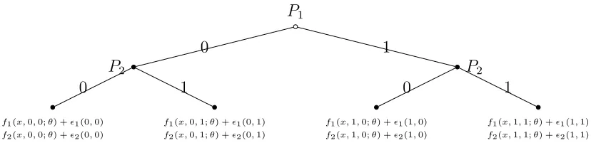
For the purpose of exposition, we provide a simple sequential entry game as an

ex-ample. There are two players who act as potential entrants in each of T markets. The

structure of this entry game is illustrated in figure a with payoffsu1 and u2 as defined in

(8)

P1

P2

f₁(x,0,0;θ) +ǫ₁(0,0)

f₂(x,0,0;θ) +ǫ₂(0,0)

0

f₁(x,0,1;θ) +ǫ₁(0,1)

f₂(x,0,1;θ) +ǫ₂(0,1)

1 0

P2

f₁(x,1,0;θ) +ǫ₁(1,0)

f₂(x,1,0;θ) +ǫ₂(1,0)

0

f₁(x,1,1;θ) +ǫ₁(1,1)

f₂(x,1,1;θ) +ǫ₂(1,1)

[image:8.595.99.513.130.246.2]

1 1

Figure a: A simple entry game

to be an equilibrium outcome, we require the following three equilibrium conditions:

u1(x,0,0, ǫ1(0,0);θ)> u1(x,1,0, ǫ1(1,0);θ) if u2(x,1,0, ǫ2(1,0);θ)> u2(x,1,1, ǫ2(1,1);θ)

u1(x,0,0, ǫ1(0,0);θ)> u1(x,1,1, ǫ1(1,1);θ) if u2(x,1,0, ǫ2(1,0);θ)≤u2(x,1,1, ǫ2(1,1);θ)

u2(x,0,0, ǫ2(0,0);θ)≤u2(x,0,1, ǫ2(0,1);θ)

(3)

The equilibrium conditions required for the other three action profiles to be equilibrium

outcomes can be formulated similarly. Since the econometrician only observes the

equi-librium outcomes but not strategies, the equiequi-librium conditions can be viewed as logical

statements that are conditional on the off equilibrium path choices, which are unobserved

by the econometrician. We make use of MINLP to handle such logical statements.

3 Preliminary

We start by providing some background to the GME approach. Also, since our GME

estimator is obtained via a (convex) MINLP, we also provide a review of the MINLP

problem.

3.1 A Basic Review of GME

(9)

measure the uncertainty (state of knowledge) we have about the occurrence of a

collec-tion of events. Let x be a random variable with possible outcomes xs, s = 1,2, . . . , n,

with probabilities αs such that

P

sαs = 1. Shannon (1948) defined the entropy of the

distribution α= (α1, ...α_n)′, as

H _{≡ −}X

s

αslnαs (4)

where 0 ln 0 _≡ 0. To recover the unknown probabilities α that characterize a given

data set,Jaynes(1957a,b) proposed maximizing entropy, subject to the available

sample-moment information and adding up constraints on the probabilities.

Within the classic ME framework, the observed moments are assumed to be exact.

To extend this approach to the problem with noise, the GME approach (developed by

Golan, Judge, and Miller (1996)) generalizes the ME approach by using a dual objective

(precision and prediction) function. We illustrate the GME approach via a linear model:

Y =Xβ+ε (5)

where Y is an N _×1 dependent variable vector, X is an N _×K matrix of explanatory

variables, β is a K_×1 a vector of parameters, and ε is an N _×1 vector of disturbance

terms. The GME estimator of β in this general linear model is derived in the following

manner. First, ˆp= (ˆp′

(10)

problem:

max

p′ k,w′i

−

K

X

k=1

p′_kln(pk)− N

X

i=1

ω_i′ln(ωi) (6)

s.t. Y =XZp+V ω

1′pk = 1, ∀k

1′_ω

i = 1, ∀i

pk>[0], ωi >0. ∀i, k.

Z and V are K _×KM and N _×N J matrices of support points for the β and ε vectors,

defined respectively, as:

Z =             

z1′ 0 ... 0

0 z2′ ... 0

. . ... .

0 0 ... z_K′

            

and V =

            

v1′ 0 ... 0

0 v2′ ... 0

. . ... .

0 0 . v_N′ .

             (7)

The M _×1 vector zk = (zk1, ...z_kM)′ is such thatz_k1 < z_k2 ≤...≤z_kM and it is assumed

that βk ∈ (zk1, z_kM) for each k

6

. The vector vi = (vi1, ...viJ)′ is such that vi1 < vi2 ≤

... _≤ viJ and it is assumed that εi ∈ (vi1, viJ) for each i. Typically, each vi1 and

viJ will be uniformly and symmetrically distributed about zero and have the same J

dimensions. The actual bounds used for a given problem depend on the observed sample

as well as any available conceptual or empirical information7

. pk = (pk1, ...p_kM)′ and

6

This parameter support is based on prior information or economic theory, for example, we might specify boundaries ofzk1= 0 andzkM = 1 when estimating the marginal propensity to consume. Without

any available prior information, we can specifyzk to be symmetric around zero, with large negative and

positive boundaries, for example,zk1=−zkM =−106.

7

(11)

ωi = (ωi1, ...ω_iJ)′ are non-negative weight vectors that sum to unity. The GME estimator

is then given by ˆβ =Zpˆ. Golan, Judge, and Miller(1996) has a rigorous discussion of this

approach and applies it to a rich scopes of econometric problems, such as dynamic models,

model selection and discrete choice-censored problems. Mittelhammer and Cardell(1997)

establish consistency and asymptotic normality results for the GME estimator under

general regularity conditions.

3.2 A Basic Review of MINLP

Our GME estimator for the sequential-move game is essentially obtained by solving a

generalized disjunctive programming problem, which can be reformulated as an MINLP

problem. Here we provide a basic review of the general structure and of existing available

algorithms for solving MINLP problems. A simple algebraic representation of an MINLP

problem is as follows:

min

{x,y} Z =f(x, y) (8)

s.t. gj(x, y)≤0, j ∈J

x_∈X, y _∈Y

wheref(_·) andg(_·) are differentiable functions,J is the index set of inequalities, andxand

y are continuous and discrete variables, respectively. In most applications the discrete

set Y is restricted to be binary. When both f(_·) and g(_·) are both convex functions,

this becomes a convex MINLP problem, which can be exactly solved via most existing

algorithms 8

. We take the technique of solving an MINLP problem as given.

(Golan, Judge, and Perloff 1997)

8

(12)

4 Estimation

In this section we first detail the assumptions required for our estimation method. We

then describe the estimator in detail before discussing its limitations and extensions.

4.1 Assumptions

We require three assumptions in order to use our estimation method. The first is

associated with the structure of the game tree, the second is associated with the ordinality

of utility, and the third is associated with the distributional properties pf the errors terms.

Assumption 1 (Exogenous Decision Order) The decision order of agents in the

sequential-move game is exogenous and known to the econometrician.

Although the exact decision order of agents is rarely observed, to estimate

sequential-move games we must assume a specific decision order.

Assumption 2 (Scale and Location Normalizations) The payoff of one action for

each player are fixed at a known constant.

From the equilibrium condition (2), any affine transformation of the payoffs does not

perturb the set of equilibria, so scale and location normalizations are necessary. The

scale normalization is subsumed in the following assumption about the distribution of

the error terms. Bajari, Hong, and Ryan (2010) argue that this restriction is similar to

the argument that we can normalize the mean utility from the outside good equal to a

constant, usually zero, in a standard discrete choice model.

(13)

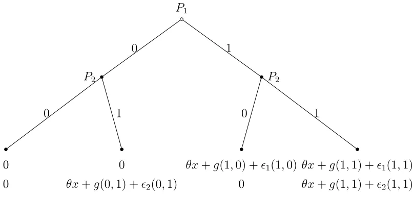
P1

P2

0 0

0

θx+g(0,1) +ǫ2(0,1)

1 0

P2

θx+g(1,0) +ǫ1(1,0)

0 0

θx+g(1,1) +ǫ1(1,1)

θx+g(1,1) +ǫ2(1,1)

[image:13.595.103.506.130.324.2]

1 1

Figure b: A Reformulated Entry Game

Assumption 3 (Regularity Conditions of Random Shocks) The random

prefer-ence shocks ǫit(a) are i.i.d, are independent of state variables, and have zero mean

and finite variance, i.e. E(ǫit(a)) = 0, E(xǫit(a)) = 0,and V ar(ǫit(a))<∞.

Thei.i.d assumption is stronger than is required for our GME estimation. Any known

heteroskedasticity and dependence among random shocks can be handled within the our

framework. We will discuss this further after presenting our estimator. Our GME

esti-mator is semiparametric in the sense that it does not impose any parametric assumption

on the random shocks.

For the purpose of exposition, we apply GME estimation under assumption 1 to 3 to

the simple entry game which was introduced in section 2. We assume that utility takes

the form:

ui(x, a, ǫi;θ) = 1(ai = 1){θx+δg(a) +ǫi(a)} (9)

(14)

The location normalization sets the utility from out of the market to 0 and scale

normalization sets the parameter δ to 1 9

. The equilibrium conditions for action profile

(0,0) to be an SPE outcomes are:

Player1: 0> θx+g(1,0) +ǫ1(1,0) if 0> θx+g(1,1) +ǫ2(1,1)

0> θx+g(1,1) +ǫ1(1,1) if 0≤θx+g(1,1) +ǫ2(1,1)

Player2: 0> θx+g(0,1) +ǫ2(0,1)

(10)

The equilibrium conditions required for the other outcomes can be similarly derived.

4.2 The Estimator

In order to use the GME framework, we need to specify the support space Z for θ

and the support space v1, v2, v3, v4 for ǫ1(1,0), ǫ1(1,1), ǫ2(0,1) and ǫ2(1,1) respectively.

Without loss of generality, all are M _× 1 vectors and v1 = v2 = v3 = v4 = v. The

corresponding probabilities are defined aspθ_{, ω}1

t, ω

2

t, ω

3

t, ω

4

t such that:

θ =

M

X

m=1

pθ_mzm (11)

ǫ1t(1,0) = M

X

m=1

ω1

tmv,ǫ1t(1,1) = M

X

m=1

ω2

tmv, ǫ2t(0,1) = M

X

m=1

ω3

tmv, ǫ2t(1,1) = M

X

m=1

ω4

tmv (12)

The entropy-information function H is defined as

H=₋

M

X

m=1

pθ_mln(pθ_m)₋

T X t=1 M X m=1 ω1

tmln(ω

1

tm)− T X t=1 M X m=1 ω2

tmln(ω

2

tm) (13)

− T X t=1 M X m=1

ω3_tmln(ω3_tm)₋

T X t=1 M X m=1

ω_tm4 ln(ω_tm4 )

9

(15)

Our GME estimator is obtained from the estimated probabilities which are the solution

to the following problem:

max {pθ

m,ωtm1 ,ω2tm,ω3tm,ωtm4 }

H subject to the corresponding constraints: (14)

If ao

t = (0,0)

0>PM

m=1p

θ

mzmxt+g(1,0) +PM_m=1ω 1

tmvm if 0>PM_m=1p

θ

tmvm

0>PM

m=1p

θ

mzmxt+g(1,1) +

PM

m=1ω 2

tmvm if 0≤

PM

m=1p

θ

mzmxt+g(1,1) +

PM

m=1ω 4

tmvm

0>PM

m=1p

θ

tmvm

(15)

If ao

t = (0,1)

0>PM

m=1p

θ

tmvm if 0>PM_m=1p

θ

tmvm

0>PM

m=1p

θ

tmvm if 0≤PM_m=1p

θ

tmvm

PM

m=1p

θ

mzmxt+g(0,1) +

PM

m=1ω 3

tmvm ≥0

(16)

If ao

t = (1,0)

PM

m=1p

θ

mzmxt+g(1,0) +

PM

m=1ω 1

tmvm ≥0

0>PM

m=1p

θ

tmvm

(17)

If aot = (1,1)

PM

m=1p

θ

tmvm ≥0

PM m=1p

θ

mzmxt+g(1,1) +

PM m=1ω

4

tmvm ≥0

(16)

and the normalization-additivity constraints:

PM

m=1p

θ m = 1

PM m=1ω

i

tm = 1,∀t∈T, ∀i∈ {1,2,3,4}

pθ m, ω

1

tm, ω

2

tm, ω

3

tm, ω

4

tm >0;∀t ∈T, m∈M

(19)

Note that for each repetition of the game, there is a unique equilibrium. Thus, the

constraints for each market are one of the four possible constraints listed in equations

(15) to (18). Our GME estimator of the structural parameterθ is

ˆ

θGM E = M

X

m=1

ˆ

pθ_mzm (20)

For this simple game, constraints (15) and (16) contain logical if-then statements

between endogenous variables. This programming is called disjunctive programming,

which can be reformulated as an MINLP. For example, consider the logical statements:

y1 <0 if x <0; y2 <0 ifx≥0 (21)

By introducing a zeroor one variable q, the statement (21) can be restated as:

x₋K(1₋q)<0; x+Kq _≥0; y1 < K(1−q); y2 < Kq; q={0,1}, (22)

where K is a positive variable which exceeds the bound of _|x_|, _|y1| and |y2|. Such

re-formulations are discussed extensively in Williams (1985) and Raman and Grossmann

(17)

By introducing such a binary variable K, our GME method can be reformulated as:

max {pθ

m,ω1tm,ω2tm,ωtm3 ,ωtm4 ,qt}

H s.t. (23)

If aot = (0,0)

PM

m=1p

θ

mzmxt+g(1,1) +

PM

m=1ω 4

tmvm ≥ −Kqt

PM

m=1p

θ

tmvm < K(1−qt)

PM

m=1p

θ

mzmxt+g(1,0) +

PM

m=1ω 1

tmvm < K(1−qt)

PM

m=1p

θ

tmvm < Kqt

0>PM

m=1p

θ

tmvm

if ao

t = (0,1)

PM

m=1p

θ

tmvm ≥ −Kqt

PM

m=1p

θ

mzmxt+g(1,1) +

PM

m=1ω 4

tmvm < K(1−qt)

PM

m=1p

θ

tmvm < K(1−qt)

PM

m=1p

θ

tmvm < Kqt

PM

m=1p

θ

mzmxt+g(0,1) +

PM

m=1ω 3

tmvm≥0

and equation (17), (18)

normalization-additvity constraints equation (19)

qt∈ {0,1}

This optimization, which can be solved via MINLP techniques, yields the estimated

(18)

Thus the estimated ˆθ can be recovered from the original reparameterization:

ˆ

θGM E = M

X

m=1

ˆ

pθ_mzm (24)

Note that if the payoff function is linear in all covariates, x, then the optimization

problem becomes a convex MINLP, since the objective entropy function is always concave.

For the game which has additional players, actions, or stages, the estimation can be easily

extended to involve more constraints.

The GME estimator proposed above essentially is a MPEC style estimator, as argued

by Su and Judd (2008), implementing asymptotic inference methods is more complex

within the MPEC framework. Computing standard errors requires the computation of

the Hessian of the objective function with respect to the structural parameters θ. Such

work seems hard due to the non-smoothness of our GME estimation.

Horowitz (1997, 1998, 2001) explains how some non-smooth estimators can be

smoothed in a way that greatly simplifies the analysis of their asymptotic distributional

properties. Smoothing our GME estimator is also possible since for most cases we can

reformulate the MINLP problem into a nonlinear programming (NLP) with

complemen-tarity constraints (MPCC). Chen and Mangasarian (1996) provides a class of smoothing

functions for nonlinear and mixed complementarity problems.

Alternatively, some recently derived resampling methods can deal with such

nonreg-ular estimators. Zeng and Lin (2008) suggests some efficient resampling procedures for

non-smooth estimators based on asymptotic expansion via empirical process arguments.

Andrews and Guggenberger(2009) also provides some efficient Hybrid and Size-Corrected

subsampling methods. We will investigate these alternative methods for inference within

our GME estimation framework in future work.

As noted above, our framework can deal with a wide range of random shock structures

(19)

considered by Maruyama (2009). Consider the simple entry game in figure.2, where the

random preference shock for player i in market t is specified as:

ǫit(a) =ωit(a) +ηi (25)

The market specific shock ηi and idiosyncratic preference shock ωit(a) are both

indepen-dently distributed across players (entrants) and markets. We can individually estimate

ωit(a) and ηi instead ofǫit(a), using an additive entropy objective function.

5 Monte Carlo

To demonstrate the performance of our estimator in small samples, we conducted two

Monte Carlo experiments using the simple sequential entry game introduced in section 2.

There are two players and each player has the following profit function:

ui(x, a, ǫi;θ) = 1(ai = 1){θ1x1+θ2x_i2−θ3x_i3+ǫ_i(a)} (26)

We definex1 ∼N(10,1), x_i2 ∼N(1,1),and x_i3 = 9(N(a)−1), whereN(a) is the number

of entrants from an action profilea. In the first experiment, the idiosyncratic error terms,

ǫit(a), are drawn from the standard normal distribution. In the second experiment, ǫit(a)

are drawn from the uniform distribution [₋1,1].

As discussed previously, our model requires both scale and location normalizations, so

we assume that θ3 = 1 and the payoffs from not entering are zero. Thus our game has

two unknown parameters: θ1 and θ2. We generated 10000 samples of size t= 25,50,100,

and 200 to assess the finite sample properties of our estimator. The true parameter vector

values were chosen as θ1 = 1 and θ2 = −1. The parameter estimates are presented in

(20)

[image:20.595.112.500.168.456.2]

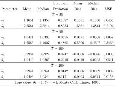
Table I: Monte Carlo Results for Normal Shocks

Standard Mean Median

Parameter Mean Median Deviation Bias Bias MSE

T = 25

θ1 1.1651 1.1350 0.1387 0.1651 0.1350 0.0465

θ2 −2.5561 −2.3814 0.8934 −1.5561 −1.3814 3.2194

T = 50

θ1 1.0471 1.0388 0.0555 0.0471 0.0388 0.0052

θ2 −1.5566 −1.4607 0.4868 −0.5566 −0.4607 0.5466

T = 100

θ1 0.9934 0.9924 0.0247 −0.0066 −0.0076 0.0006

θ2 −1.0449 −1.0265 0.2215 −0.0449 −0.0265 0.0511

T = 200

θ1 0.9944 0.9941 0.0142 −0.0056 −0.0059 0.0002

θ2 −1.0403 −1.0344 0.1171 −0.0403 −0.0344 0.0153

True value: θ1 = 1, θ2 =−1; Monte Carlo Times: 10000

cand d.

The results are encouraging even in smaller samples sizes; the payoff parameters are

estimated close to their true values, and as the sample size increases, the estimates become

more precise. Parameter θ1 is estimated more precisely. This is mainly because θ1 has a

larger influence over equilibrium thanθ2, since θ1 interacts with a covariate with a higher

mean than θ2 does. In an extremely small sample, the variation in θ2 may not generate

sufficient variation in equilibrium to be estimated precisely but this problem disappears

as the sample size becomes larger.

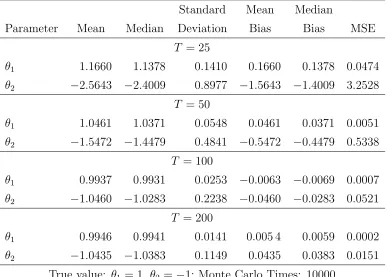
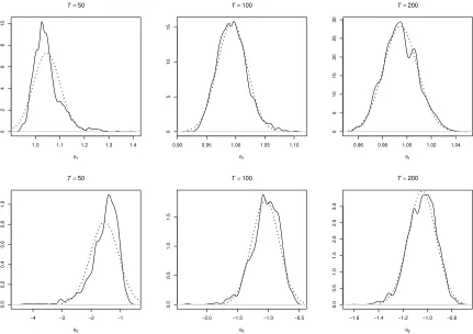
The second simulation shows that our GME estimator can handle non-normal errors.

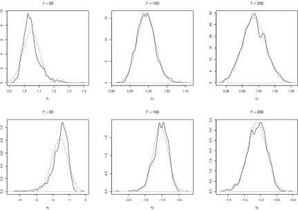
The empirical distributions of the parameter estimates shown in figures 3 and 4 also show

(21)

[image:21.595.112.499.323.600.2]

Table II: Monte Carlo Results for Uniform Shocks

Standard Mean Median

Parameter Mean Median Deviation Bias Bias MSE

T = 25

θ1 1.1660 1.1378 0.1410 0.1660 0.1378 0.0474

θ2 −2.5643 −2.4009 0.8977 −1.5643 −1.4009 3.2528

T = 50

θ1 1.0461 1.0371 0.0548 0.0461 0.0371 0.0051

θ2 −1.5472 −1.4479 0.4841 −0.5472 −0.4479 0.5338

T = 100

θ1 0.9937 0.9931 0.0253 −0.0063 −0.0069 0.0007

θ2 −1.0460 −1.0283 0.2238 −0.0460 −0.0283 0.0521

T = 200

θ1 0.9946 0.9941 0.0141 0.005 4 0.0059 0.0002

θ2 −1.0435 −1.0383 0.1149 0.0435 0.0383 0.0151

(22)

0.9 1.0 1.1 1.2 1.3 1.4

0

2

4

6

8

10

T=50

θ1

0.90 0.95 1.00 1.05 1.10

0

5

10

15

T=100

θ1

0.96 0.98 1.00 1.02 1.04

0

5

10

15

20

25

30

T=200

θ1

−4 −3 −2 −1 0

0.0

0.2

0.4

0.6

0.8

1.0

T=50

θ2

−2.0 −1.5 −1.0 −0.5

0.0

0.5

1.0

1.5

T=100

θ2

−1.4 −1.2 −1.0 −0.8 −0.6

0.0

0.5

1.0

1.5

2.0

2.5

3.0

3.5

T=200

[image:22.595.91.522.284.588.2]

θ2

(23)

1.0 1.1 1.2 1.3 1.4

0

2

4

6

8

10

T=50

θ1

0.90 0.95 1.00 1.05 1.10

0

5

10

15

T=100

θ1

0.96 0.98 1.00 1.02 1.04

0

5

10

15

20

25

30

T=200

θ1

−4 −3 −2 −1

0.0

0.2

0.4

0.6

0.8

1.0

T=50

θ2

−2.0 −1.5 −1.0 −0.5

0.0

0.5

1.0

1.5

T=100

θ2

−1.6 −1.4 −1.2 −1.0 −0.8

0.0

0.5

1.0

1.5

2.0

2.5

3.0

T=200

[image:23.595.91.522.284.588.2]

θ2

(24)

6 Conclusion

In this paper, we developed a data-constrained GME estimator for the discrete

sequential-move game of perfect information. By directly using the data-constraints which are

im-plied by the equilibrium conditions, we avoid the multidimensional integration which

always makes such estimation intractable. Moreover, in contrast to existing estimators

for general complete information games, our GME estimator requires no parametric

as-sumption about the distribution of the random shocks. We formulate the estimation as

a (convex) mixed-integer nonlinear optimization problem. The estimation can be easily

implemented on optimization software with high-level interfaces such as GAMS or AMPL.

The model is identified with only weak scale and location normalizations. Monte Carlo

evidence demonstrates that the estimator can perform well in moderately sized samples.

References

Aguirregabiria, V., and P. Mira (2007): “Sequential Estimation of Dynamic

Dis-crete Games,” Econometrica, 75, 1–53.

Andrews, D. W. K., and P. Guggenberger (2009): “Hybrid and Size-Corrected

Subsampling Methods,” Econometrica, 77(3), 721–762.

Bajari, P., H. Hong, J. Krainer, and D. Nekipelov (2010): “Estimating Static

Models of Strategic Interactions,” Journal of Business and Economic Statistics.

Bajari, P., H. Hong,and S. Ryan(2010): “Identification and Estimation of a Discrete

Game of Complete Information,” Econometrica.

Berry, S., and E. Tamer (2007): “Identification in Models of Oligopoly Entry,” in

Advanced in Economics and Econometrics: Theory and Application, vol. II, chap. 2, pp. 46–85. Cambridge University Press.

Berry, S. T. (1992): “Estimation of a Model of Entry in the Airline Industry,”

(25)

Bonami, P., M. Kilinc, and J. Linderoth (2009): “Algorithms and Software for Convex Mixed Integer Nonlinear Programs,” Discussion paper, University of Wisconsin Madison.

Bresnahan, T. F., and P. C. Reiss (1990): “Entry in Monopoly Markets,”Review of

Economic Studies, 57, 531–553.

(1991): “Empirical models of Discrete Games,” Journal of Econometrics, 48, 57–81.

Campbell, R. C.,andR. C. Hill(2001): “Maximum Entropy Estimation in Economic

Models with Linear Inequality Restrictions,” Working Paper.

Chen, C., and O. L. Mangasarian (1996): “A Class of Smoothing Functions for

Nonlinear and Mixed Complementarity Problems,” Computational Optimization and Applications, 5(2), 97–138.

Golan, A., G. Judge, and J. Miller (1996): Maximum Entropy Econometrics:

Ro-bust Estimation with Limited Data. John Wiley & Sons, New York.

Golan, A., G. Judge, and J. Perloff (1997): “Estimation and Inference with

Cen-sored and Ordered Multinomial Response Data,” Journal of Econometrics, 79(1), 23– 51.

Golan, A., L. S. Karp, and J. Perloff (1998): “Estimating a Mixed Strategy:

United and American Airlines,” Working Paper.

Golan, A., L. S. Karp, and J. M. Perloff (2000): “Estimating Coke’s and Pepsi’s

Price and Advertising Strategies,” Journal of Business and Economic Statistics, 18(4), 398–409.

Golan, A., J. M. Perloff, and E. Z. Shen (2000): “Estimating a Demand System

with Nonnegativity Constraints: Mexican Meat Demand,” Working Paper.

Horowitz, J. L. (1997): “Bootstrap Methods in Econometrics: Theory and Numerical

Performance,” inAdvances in Economics and Econometrics: Theory and Applications: Seventh World Congress, ed. by D. M. Kreps, and K. F. Wallis, vol. III, chap. 7, pp. 188–222. Cambridge University Press.

Horowitz, J. L. (1998): “Bootstrap Methods for Median Regression Models,”

(26)

(2001): “The Bootstrap,” in Handbook of Econometrics, ed. by J. Heckman,and

E. Leamer, vol. 5, pp. 3159–3228. Elsevier Science, The Netherlands.

Jaynes, E. T. (1957a): “Information Theory and Statistical Mechanics,” Physics

Re-views, 106, 620–630.

(1957b): “Information Theory and Statistical Mechanics, II,” Physics Reviews, 108, 171–190.

Jouneau-Sion, F., and O. Torres (2006): “MMC techniques for limited dependent

variables models: Implementation by the branch-and-bound algorithm,” Journal of Econometrics, 133(2), 479–512.

Lee, L. (1995): “Asymptotic Bias in Simulated Maximum Likelihood Estimation of

Discrete Choice Models,” Econometric Theory, 11(3), 437 – 483.

Maruyama, S.(2009): “Estimating Sequential-move Games by a Recursive Conditioning