Control and Synchronization with Known and Unknown Parameters

(1)

http://dx.doi.org/10.4236/am.2016.73026

Control and Synchronization with Known

and Unknown Parameters

Maysoon M. Aziz, Saad Fawzi Al-Azzawi

Department of Mathematics, College of Computer Sciences and Mathematics, University of Mosul, Mosul, Iraq

Received 6 January 2016; accepted 26 February 2016; published 29 February 2016

This work is licensed under the Creative Commons Attribution International License (CC BY).

http://creativecommons.org/licenses/by/4.0/

Abstract

In this paper, we consider the chaos control for 4D hyperchaotic system by two cases, known & unknown parameters based on Lyapunov stability theory via nonlinear control. We find that there are two cofactors that have an effect on determining any case to achieve the control, the two co-factors are proposed in the control and the matrix that produce from the time derivative of Lya-punov function. In adding, we find some weakness cases in LyaLya-punov stability theory. For this reason, we design with only one controller and perform a simple change in this control in order to recognize the difference between these cases although all of the controllers are almost similar.

Keywords

4D Hyperchaotic System, Control, Synchronization, Lyapunov Stability Theory, Nonlinear Control Method

1. Introduction

Chaos phenomenon was firstly observed by Lorenz in 1963 [1]-[4]. Chaos control is one of the chaos phenome-na, which contains two aspects, namely, chaos control and chaos synchronization [5]. Chaos control and chaos synchronization were once believed to be impossible until the 1990s when Ott et al. developed the OGY method to suppress chaos. Pecora and Carroll introduced a method to synchronize two identical chaotic systems with different initial conditions [2] [5]-[12].

Many different techniques for chaos control and synchronization have been developed, such as a linear feedback method, active control approach, adaptive technique, time delay feedback approach, and back step-ping method. Among them, nonlinear control is an effective method to control chaos [2]-[4] [6] [7] [9] [12]-[15].

(2)

another some achieved control and synchronization with known parameters only. In this paper, we perform chaos control for two cases and we find that the proposed control plays an important and active role to determine the case as well as the matrix of time derivative for Lyapunov function, where the strategy of this paper is based on designing only one control. We also perform some simple change into this control, study probability of sup-pression for each control by using Lyapunov stability theory and get three cases. In first case, we can achieve control directly when parameters are unknown; in second type, we need to modify in order to achieve control with known parameters; finally in third type, it is imposable to perform the control.

Although the accuracy of Lyapunov stability theory is not neglected and the nonlinear parts have been suc-cessful in the treatment of the first two types, but it failed to treat the third type. So, we refuge to use the linear approximation method to treat the problem and the weaknesses.

Briefly, this study poses three fundamental questions. First, when can we achieve chaos control with known parameters? Second, when can we achieve chaos control with unknown parameters? And third, how can we dis-tinguish between these two cases? This paper begins with the suggestion of a new method that will answer these questions.

2. Problem Formulation and Our Methodology

In this section, we describe the problem formulation for the chaos control and chaos synchronization for hyper-chaotic systems and our methodology using nonlinear control by basing on the Lyapunov stability theory.

Let us consider the hyperchaotic system in the following form:

( )

X =AX +f X (1) where

( )

[

1, 2, ,

]

T 1

n n

X t = x x  x ∈R× is the state of the system, A=

( )

aij _{n n}_× is the matrix of the system para-meters, and _f :_Rn_→_Rn_{is the nonlinear part of the system, this nonlinear part can represent by many}

formu-lations, one of these formulations as f X

( )

=xBX, B=

( )

bij _{n n}_× is the matrix of the nonlinear part of the sys-tem (1),

If we add the controller

[

1, 2, ,

]

T 1 n n

U= u u  u ∈R × into the system (1), then the controlled system is given by:

( )

X =AX + f X +U (2) The aim of the control problem is to design a feedback controller U such that lim

( )

0

t→∞ X t = .

But, in synchronization problem we needed two system, drive system and response system. Let us consider the system (1) as the drive system and the response system is given by the following forms:

( )

Y=CY+g Y +U (3) where

( )

[

1, 2, ,

]

T 1

n n

Y t = y y  y ∈R × is the state of the system, C=

( )

cij _{n n}_× is the matrix of the system para-meters, and g R: n →Rn is the nonlinear part of the system. If A=C and f X

( )

=g Y

( )

, then X and Y are the states of two identical (nearly identical) systems. If A≠C and/or f X

( )

≠g Y

( )

, then X and Y are the states of two different systems.

The error dynamics for the synchronization can be expressed as

( )

e=CY+g Y −AX− f X +U (4) where e= −Y X. The objective of synchronization problem is to find a controller U such that lim

( )

0

t→∞ e t = .

It is clear that the problem of synchronization between the drive and response systems is replaced by the equivalent problem of stabilizing the system (4) using a suitable choice of the control U [10].

In unknown parameter, we assume that the Lyapunov function is always formed as V X

( )

= X PXT

(

)

diag 1 2 ,1 2 , ,1 2

(3)

para-meter. But in known parameters, the matrix Q is not diagonal. So, we needed to modify the matrix P in order to make the matrix Q is diagonal matrix. Consequently, we ensure to get negative definite function i.e. V X

( )

<0. By this difference we can recognize between two cases (chaos control with known and unknown parameters) based on the Lyapunov stability theory.

According to the above discussion, and based on Lyapunov stability theory, we can obtain the following con-clusion.

Corollary 1. To determine the chaos control with known and unknown parameters we based on two cofators: a) Controller design, b) the matrix Q.

If we get the matrix Q as:

a) Identity or diagonal matrix. Then, we choose chaos control with unknown parameters; b) not diagonal ma-trix. Then, we choose chaos control with known parameters (in order to translate not diagonal matrix to diagonal we must give the value of parameters and make modify on the matrix P).

3. Chaos Control

In this section, we achieve controlling problems with known and unknown parameters for the hyperchaotic sys-tem [3] [4], which is described by the following nonlinear differential equation

(

)

x a y x

y cx xz w

z xy bz

w dy

 = −

 ₌ ₋ ₊



 ₌ ₋

  = − 

   

(5)

where

(

x y z u, , ,

)

∈R4, and a b c d, , , ∈R are positive constant parameters, this system is hyperchaotic system when a=10, b=8 3, c=28 and d=10, and has only one equilibrium O

(

0, 0, 0, 0

)

.

In order to control above hyperchaotic system to zero, the feedback controllers of u u u1, 2, 3 and u4 are added to the hyperchaotic system (5) according to the formulation (2). Then, the controlled hyperchaotic system is given by:

(

)

1

2

3

4

x a y x u

y cx xz w u

z xy bz u

w dy u

= − +



 ₌ ₋ _{+ +}



 ₌ _{− +}



 = − + 

   

(6)

in which a b c, , and d are unknown parameters, and u u u u1, 2, 3, 4 are feedback controllers to be designed. 3.1. Controlling Hyperchaotic System (6) with Unknown Parameters

In the following theorem, we proposed nonlinear control with unknown parameters to control system (6).

Theorem 1. The controlled hyperchaotic system (6) will achieve globally asymptotically stable with the fol-lowing nonlinear controllers:

(

)

(

)

(

)

(

)

1

2

3

4

1

u a x

u a c x y

u b z

u d y w

= −

 

= − + −

 

= −



 = − −



(7)

Proof. Substituting the controllers (7) in the system (6), we have

x x ay

y ax y xz w

z z xy

w y w

= − + 

 = − − − + 

 = − + 

 = − − 

   

(4)

According to the formulation (1), the above system can be rewritten as:

1 0 0 0 0 0 0

1 0 1 0 0 1 0

0 0 1 0 0 1 0 0

0 1 0 1 0 0 0 0

x a x x

y a y y

x

z z z

w w w

−

         

  ₋ ₋     ₋   

  ₌   ₊    

   −       

   ₋ ₋       

         

   

(9)

To achieve the control of this system, there are two methods, Lyapunov stability theory and linearization me-thod.

Based on the Lyapunov stability theory and corollary 1, we construct the following Lyapunov candidate func-tion

( )

T

V X =X PX (10)

where P=diag 1 2,1 2,1 2,1 2

(

)

and every diagonal matrix with positive diagonal elements is a positive definite. So V x

( )

is also a positive definite function.

Now, by controllers (7), the time derivative of the Lyapunov function is:

( )

2 2 2 2 T

V X = − −x y −z −w = −X QX (11)

Here Q=I4 is identity matrix and according to corollary 1. We can achieve chaos control with unknown parameters, and every identity matrix is positive definite. So, we have V x

( )

is a negative definite function. Hence, the controlled system (6) can asymptotically converge to the unstable equilibrium with the controllers (7).

Also, by using the linearization method, we have the characteristic equation as:

(

λ₊₁

)

λ3₊₃λ2₊

(

_a2₊₄

)

λ₊_a2₊₂₌₀

  (12)

To solve this equation with unknown parameters, we needed to analytically (Theoretical) methods such that Gardan method and Routh-Hurwitz method, while using the numerical methods when we knew these parame-ters.

By Routh-Hurwitz method, Equation (12) has all roots with negative real parts if and only if a2+ >2 0 and 2

5 0

a + > . So, it is clear that satisfies the conditions for this method. Consequently, according to two methods (Lyapunov stability theory, linearization method), system (6) with control (7) is globally asymptotically stable. The proof is complete.

3.2. Controlling Hyperchaotic System (6) with Known Parameters

If we make simple change into control (7) i.e. change only second equation to become the following forms:

(

)

(

)

(

)

1

2

3

4 1

2

1

u a x

u cx y

u b z

u d y w

 = −



= − − 

 = − 

 = − −



(13)

and used the same of the Lyapunov function in Equation (10). Then, we get the time derivative for the Lyapunov function as the following:

( )

2 2 2 2

(

)

T

1

V X = − −x y −z −w + a c xy− = −X Q X (14)

where

(

)

(

)

1

1 2 0 0

2 1 0 0

0 0 1 0

0 0 0 1

a c a c

Q

− −

 

_{− −} 

 

=_ _

 

(5)

By this control, we obvious the matrix Q1 is not diagonal and contains parameters. Here are two ways to tell if it’s above matrix is a positive definite, in the first way, we can use determinants test or pivot test without we know the value of these parameters while in the second way (based on corollary 1.), We must give the value of these parameters in order to translate the matrix Q1 to the diagonal matrix. Consequently, the control problem with unknown parameters is replaced by the equivalent problem of controlling with known parameters. But if we substitute the value of these parameters as a=10, b=8 3, c=28 and d=10 in the matrix Q1 we get a matrix with a negative definition and the method is failing, For treatment this problem we must choose a suitable Lyapunov function or modify the matrix P to make the matrix Q1 is a positive definite, and the following theorem explains this modification.

Theorem 2. The controlled hyperchaotic system (6) with nonlinear control (13) is globally asymptotically stable.

Proof. The system (6) with control (13) becomes:

x x ay

y cx y xz w

z z xy

w y w

= − + 

 = − − − + 

 = − + 

 = − − 

   

(15)

This system can be reformulated in the following form:

1 0 0 0 0 0 0

1 0 1 0 0 1 0

0 0 1 0 0 1 0 0

0 1 0 1 0 0 0 0

x a x x

y c y y

x

z z z

w w w

−

         

  ₋ ₋     ₋   

  ₌   ₊    

   −       

         

− −

         

   

(16)

Now, according to the Lyapunov second method, Let us modify the Lyapunov function by the following form i.e. modify the matrix p to get the matrix p1:

(

)

(

)

(

)

T 2 2 2 2

1 1 2 10 28 10 28 10 28

V =X P X = _x + y + z + w _ (17)

where 1

1 2 0 0 0

0 5 28 0 0

0 0 5 28 0

0 0 0 5 28

P

 

 

=

 

 

is a diagonal matrix

So, we have the time derivative of the Lyapunov function as:

(

)

(

)

(

)

2 2 2 2 T

2 10 28 10 28 10 28

V= − −x y − z − w = −X Q X (18)

where 2

1 0 0 0

0 10 28 0 0

0 0 10 28 0

0 0 0 10 28

Q

 

 

=

 

 

is also diagonal matrix

Consequently, we translate the matrix Q1 (not diagonal) to matrix Q2 (diagonal) for the same control (13) after we input the value of parameters, at the same time we modified the matrix p to become the matrix p1. Then, we get V<0, which gives asymptotic stability of the system (6) by Lyapunov stability theory. This means that the controller proposes is achieved the suppressed of system (6).

On the other hand, the control problem for a system (6) with control (13) can be achieved by linearization method. Then, we have the characteristic equation forms:

(

)

3 2

(

)

1 3 ac 4 ac 2 0

λ+ _λ + λ + + λ+ + _= (19)

(6)

(

)

3 2

1 3 284 282 0

λ+ _λ + λ + λ+ _= (20)

and the roots of the above equation are λ1,2= −1,λ3,4= − ±1 16.7631i. Therefore, all roots with negative real

parts. Consequently, we achieved the control system (6) by linearization method, the proof is complete.

Remark1. We founded the roots of Equation (20) by numerical methods. Also, we can use Gardan and Routh-Hurwitz methods for it.

Obviously, from theorem 1, the matrix P=diag 1 2,1 2,1 2,1 2

(

)

with control (7) is succeed to achieve the control directly while in theorem 2, we needed to modify the matrix P to become P₁=diag 1 2, 5 28, 5 28, 5 28

(

)

in order to equivalent the control (13), but in some time, it is impossible to modify the matrix P to ensure the convergence of the zero by using Lyapunov stability theory which is refer to the weakness for this method and the following theorem explain this case.

Theorem 3. If the nonlinear controllers are proposed as:

(

)

(

)

(

)

(

)

1

2

3

4

1

3 1

u a x

u a c x y

u b z

u d y w

= −

 

= − + −

 

= −



 = − −



(21)

i.e. simple change in four equation for control (7). Then, the zero solution of the controlled hyperchaotic system (6) can’t convergent by Lyapunov stability theory and is globally asymptotically stable by linearization method.

(

2 1

)

x x ay

y ax y xz w

z z xy

w d y w

= − + 

 = − − − + 

 = − + 

 = − −



   

(22)

Also system (22) can be rewritten (According to the formulation (1)) as:

1 0 0 0 0 0 0

1 0 1 0 0 1 0

0 0 1 0 0 1 0 0

0 2 1 0 1 0 0 0 0

x a x x

y a y y

x

z z z

w d w w

−

         

  ₋ ₋     ₋   

  ₌   ₊    

   −       

   ₋ ₋       

         

   

(23)

To check the control of this system by using Lyapunov stability theory, we can construct a Lyapunov function as

( )

T

V X =X PX and then we have the time derivative as the following:

( )

2 2 2 2 T

3 2

V X = − −x y −z −w + dyw= −X Q X (24)

Here 3

1 0 0 0

0 1 0

0 0 1 0

0 0 1

d Q

d

 

 ₋ 

 

=

 

 ₋ 

 

is not diagonal matrix and contains a parameter

So it is impossible to turn this matrix Q3 to a diagonal matrix with positive parameter, and we have V x

( )

is a positive definite function and failed this method to control (21). In order to overcome this problem, we used the linearization method. Then, we have the characteristic equation forms:

(

)

3 2

(

2

)

2

1 3 a 2d 4 a 2d 2 0

λ+ _λ + λ + − + λ+ − + _= (25)

Since the parameters are known, we have

(

)

3 2

1 3 84 82 0

(7)

And the roots of this equation are λ1,2 = −1,λ3,4= − ±1 9i therefore we succeed to achieve the chaos control for

system (6) with control (21) by linearization method only.

4. Chaos Synchronization

In this section, we consider the synchronization problem of the hyperchaotic system (5) with known and un-known parameters using corollary 1. and how we can apply this corollary to determine between them,

Let us consider the hyperchaotic system (5) as the drive system, and the controlled hyperchaotic system (6) as the response system.

Subtracting system (5) from the system (6), we obtain the error dynamical system between the drive system and the response system which is given by:

(

)

(

)

1 2 1 1

2 1 4 1 3 3 2

3 3 1 2 2 1 3

4 2 4

e a e e u

e c z e e e e xe u

e be e e xe ye u

e de u

 = − +



= − + − − +

 

= − + + + +



 = − + 

   

(27)

where e1= −x1 x e, 2= y1−y e, 3= −z1 z and e4=w1−w.

System (27) describes the error dynamics according to formulation 4.

4.1. Chaos Synchronization of System (27) with Unknown Parameters

Theorem 4. The zero solution of the error dynamical system (27) is asymptotically stable if nonlinear control is designed as following:

(

)

(

)

(

)

(

)

1 1 2

2 2 3 1

3 3 2 1

4 2 4

1

u a e a c e

u e xe ze

u b e xe ye

u d e e

= − − +



 _{= − +} ₊



 = − − −



 = − −



(28)

1 1 2

2 1 2 4 1 3

3 3 1 2

4 2 4

e e ce

e ce e e e e

e e e e

e e e

= − − 

 = − + − 

 = − + 

 = − − 

   

(29)

According to the formulation (1), the above system can be rewritten as:

1 1 1

2 2 2

1

3 3 3

4 4 4

1 0 0 0 0 0 0

1 0 1 0 0 1 0

0 0 1 0 0 1 0 0

0 1 0 1 0 0 0 0

e c e e

e

e e e

− −

       

   ₋    ₋  

 ₌  ₊   

   −     

   ₋ ₋     

   

     

   

(30)

Based on the Lyapunov stability theory, we construct the following Lyapunov candidate function

( )

2 2 2 2 T

1 2 3 4

1 2

V e = _e + + +e e e _=e Pe (31)

And the time derivative of the Lyapunov function is:

( )

2 2 2 2 T

1 2 3 4

V X = − − − −e e e e = −e Qe (32)

(8)

( )

V e is a negative definite function. Hence, the system (27) can asymptotically converge to the unstable equi-librium with the controllers (28).

As well, by using the linearization method, we have the characteristic equation as:

(

)

3 2

(

2

)

2

1 3 c 4 c 2 0

λ+ _λ + λ + + λ+ + _= (33)

By Routh-Hurwitz method, Equation (33) has all roots with negative real parts if and only if 2 2 0 c + > and 2

5 0

c + > . So, it is clear that satisfies the conditions for this method. Consequently, according to two methods (Lyapunov stability theory, linearization method) system (27) with control (28) is globally asymptotically stable, the proof is completed.

4.2. Chaos Synchronization of System (27) with Known Parameters

Based on the previously discussed in Section 3 to make simple change into a new control (change only in first equation for control 28) to become as:

(

)

(

)

(

)

1 1 2

2 2 3 1

3 3 2 1

4 2 4

1 3

1

u a e ae

u e xe ze

u b e xe ye

u d e e

= − −

 

= − + +



 = − − −



 = − −



(34)

and used the same of the Lyapunov function in Equation (31). Then, we take the time derivative for the Lyapu-nov function as the following:

( )

2 2 2 2

(

)

T

1 2 3 4 2 1 2 4

V e = − − − − −e e e e a c e e− = −e Q e (35)

where

(

)

(

)

4

1 2 2 0 0

2 2 1 0 0

0 0 1 0

0 0 0 1

a c a c

Q

−

 

 ₋ 

 

=_ _

 

 

Obviously, the matrix Q4 is not diagonal, and contains parameters. Therefore, we can achieve chaos control with known parameters according to corollary 1, and we must modify the matrix P in order to become the matrix

4

Q is a positive definite, and the following theorem treated this case.

Theorem 5. The error dynamical system (27) with control (34) is globally asymptotically stable.

Proof. The system (27) with control (34) becomes as:

1 1 2

2 1 2 4 1 3

3 3 1 2

4 2 4

2

e e ae

e ce e e e e

e e e e

e e e

= − − 

 = − + − 

 = − + 

 = − − 

   

(36)

1 1 1

2 2 2

1

3 3 3

4 4 4

1 2 0 0 0 0 0 0

1 0 1 0 0 1 0

0 0 1 0 0 1 0 0

0 1 0 1 0 0 0 0

e a e e

e c e e

e

e e e

− −

       

   ₋    ₋  

 ₌  ₊   

   −     

       

− −

   

     

   

(37)

Now, according to the Lyapunov second method, Let us modify the Lyapunov function of the following form:

( )

T 2 2 2 2

2 1 2 14 10 1 2 3 4

(9)

where 2

7 10 0 0 0

0 1 2 0 0

0 0 1 2 0

0 0 0 1 2

P       =      

is a diagonal matrix

So, we have the time derivative of the Lyapunov function as:

( )

2 2 2 2 T

1 2 3 4 5

14 10

V e = − e − − −e e e = −e Q e (39)

where 5

14 10 0 0 0

0 1 0 0

0 0 1 0

0 0 0 1

Q       =      

is also diagonal matrix

We translate the matrix Q4 (not diagonal) to matrix Q5 (diagonal) for the same control (34) after we input the value of parameters at the same time we modified the matrix p to become the matrix p3. Then we get V<0 which gives asymptotic stability of the system (27) by Lyapunov stability theory. This means that the controller proposes is achieved the suppressed of system (27).

On the other hand, the control problem for a system (27) with control (34) can be achieved by linearization method. Then, we have the characteristic equation forms:

(

)

3 2

(

)

(

)

1 3 2 ac 2 2 ac 1 0

λ+ _λ + λ + + λ+ + _= (40)

(

)

3 2

1 3 564 562 0

λ+ _λ + λ + λ+ _= (41)

And the roots of this equation are λ1,2 = −1,λ3,4= − ±1 23.6854i therefore we succeed to achieve the

syn-chronization of the drive system (5) and the response system (6).

In adding, if we choose nonlinear control (simple change into four equations for control (34)) as:

(

)

(

)

1 1 2

2 2 3 1

3 3 2 1

4 4

1 3

1

u a e ae

u e xe ze

u b e xe ye

u e  = − −  _{= − +} ₊   = − − −   = −  (42)

with the matrix p then we have the matrix

(

)

(

)

(

)

(

)

6

1 2 2 0 0

2 2 1 0 1 2

0 0 1 0

0 1 2 0 1

a c

a c d

Q d  −   ₋ ₋    =    ₋     

To translate the matrix Q6 into diagonal matrix we must modify the matrix p in the following form

(

)

3 diag 14 20 ,1,1,1 20

p = then we have

( )

2 2 2 2 T

1 2 3 4 7

28 20 1 10

V e = − e − − −e e e = −e Q e (43)

where               = 10 / 1 0 0 0 0 1 0 0 0 0 1 0 0 0 0 10 14 7

Q is also diagonal matrix.

Obviously, from theorem 4, we can perform the controlling of error dynamics system (27) by using controller (28) with matrix p directly, while in theorem 5 we must modify the matrix P to become

(

)

2 diag 7 10,1 2,1 2,1 2

(10)

the matrix P to guarantee the convergent to the zero by using Lyapunov stability theory and the following theo-rem to explain this case.

Theorem 6. If the nonlinear controllers are proposed as:

(

)

(

)

(

)

(

)

1 1 2

2 2 3 1

3 3 2 1

4 2 4

1

2 1

u a e a c e

u e xe ze

u b e xe ye

u d e e

= − − +

 

= − + +



 = − − −



 = − −



(44)

We multiplied the parameter d by number 2 in equation four for control (28). Then, it is impossible to perform the synchronization by Lyapunov stability theory.

Proof. The system (27) with control (44) becomes as

(

)

1 1 2

2 1 2 4 1 3

3 3 1 2

4 1 2 4

e e ce

e ce e e e e

e e e e

e d e e

= − − 

 = − + − 

 = − + 

 = − − −



   

(45)

1 1 1

2 2 2

1

3 3 3

4 4 4

1 0 0 0 0 0 0

1 0 1 0 0 1 0

0 0 1 0 0 1 0 0

0 1 0 1 0 0 0 0

e c e e

e

e e e

e d e e

− −

       

   ₋    ₋  

 ₌  ₊   

   −     

       

− −

   

     

   

(46)

Now, to check the control of this system by using Lyapunov stability theory, we can construct a Lyapunov function as V e

( )

=e PeT and then we have the time derivative as the following:

( )

2 2 2 2 T

1 2 3 4 2 4 8

V e = − − − − +e e e e de e = −e Q e (47)

Here, 8

1 0 0 0

0 1 0

0 0 1 0

0 0 1

d Q

d

 

 ₋ 

 

=

 

 ₋ 

 

is not diagonal matrix and contains a parameter

So it is impossible to transient the matrix Q8 into a diagonal matrix with positive parameter, and we have

( )

V e is a positive definite function and failed this method to control (44). In order to overcome this weakness, we used the linearization method. Then, we have the characteristic equation forms:

(

λ₊₁

)

λ3₊₃λ2₊

(

_c2_{− +}_d ₄

)

λ₊_a2_{− +}_d ₂₌₀

  (48)

(

)

3 2

1 3 778 776 0

λ+ _λ + λ + λ+ _= (49)

and the roots of this equation are λ1,2 = −1,λ3,4= − ±1 27.8388i therefore we succeed to achieve the chaos control

for system (6) with control (44) by linearization method only.

(11)

[image:11.595.147.504.79.351.2]

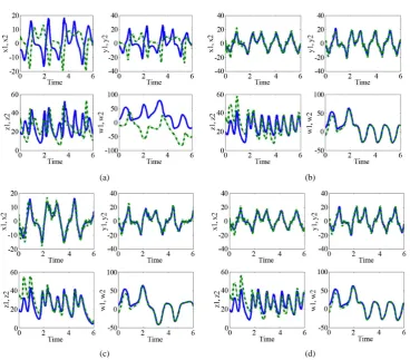
Figure 1. The attractor of space system (5) in x-y-w (a) Before control, (b) with controller (7), (c) with controller (13) (d) with controller (21).

(a) (b)

(c) (d)

[image:11.595.129.498.373.696.2]

(12)

system (5) and the response system (6) with control (28), (34) and control (44) respectively.

5. Conclusions

In this paper, we study the chaos control for 4D hyperchaotic system based on Lyapunov stability theory, where this method is effective and accurate in finding stability of systems, and in view of dealing with nonlinear parts of systems and not neglecting those parts which support the strength and accuracy.

Nevertheless, it loses this property in some time. As the case of the system in this paper, we design the control to ensure the survival of nonlinear parts in the system. And in some cases, it can suppress without knowing the parameters of the system and the other cases. We must know that the parameters and third case can’t be sup-pressed. Then, the Lyapunov stability theory will be failed in sometimes. Therefore, we use the linear approxi-mation method to ensure the validity of this proposed control. We have succeeded in achieving control, and we find that the simple difference in the control is responsible to get these three cases. Through this method, we can treat every case when the nonlinear parts have no effect on the system. Finally, numerical simulations show the effectiveness of the proposed chaos control and synchronization schemes.

References

[1] Al-Azzawi, S.F. (2012) Stability and Bifurcation of Pan Chaotic System by Using Routh-Hurwitz and Gardan Method.

Applied Mathematics and Computation, 219, 1144-1152. http://dx.doi.org/10.1016/j.amc.2012.07.022

[2] Aziz, M.M. and Al-Azzawi, S.F. (2015) Control and Synchronization of a Modified Hyperchaotic Pansystem via Ac-tive and AdapAc-tive Control Techniques. Computational and Applied Mathematics Journal, 1, 151-155.

http://www.aascit.org/journal/cam

[3] Jia, Q. (2008) Hyperchaos Synchronization between Two Different Hyperchaotic Systems. Journal of Information and Computing Science, 3, 73-80.

[4] Lu, D., Wang, A. and Tian, X. (2008) Control and Synchronization of a New Hyperchaotic System within Known Pa-rameters. International Journal of Nonlinear Science, 6, 224-229.

[5] Cai, G. and Tan, Z. (2007) Chaos Synchronize of a New Chaotic System via Nonlinear Control. Journal of Uncertain Systems, 1, 235-240. http://www.jus.org.uk

[6] Ahmad, I., Saaban, A.B., Ibrahim, A.B. and Shahzad, M. (2015) A Research on Synchronization of Two Novel Chao-tic System Based on Nonlinear Active Control Algorithm. Engineering, Technology & Applied Science Research, 5, 739-747.

[7] Aziz, M.M. and Al-Azzawi, S.F. (2015) The Relationship between Feedback Controller Numbers and Speed of Con-vergent in Control and Synchronization via Nonlinear Control. International Journal of Electrical and Electronic Sci- ence, 2, 374-380. http://www.aascit.org/journal/ijees

[8] Chen, C., Fan, T. and Wang, B. (2014) Inverse Optimal Control of Hyperchaotic Finance System. World Journal of Modelling and Simulation, 10, 83-91.

[9] Zhu, C. (2010) Control and Synchronize a Novel Hyperchaotic System. Applied Mathematics and Computation, 216, 276-284. http://dx.doi.org/10.1016/j.amc.2010.01.053

[10] Xu, J., Cai, G. and Zheng, S. (2009) Adaptive Synchronization for an Uncertain New Hyperchaos Lorenz System. In-ternational Journal of Nonlinear Science, 8, 117-123.

[11] Yassen, M.T. (2003) Adaptive Control and Synchronization of a Modified Chua’s Circuit System. Applied Mathemat-ics and Computation, 135, 113-128. http://www.elsevier.com/locate/amc

http://dx.doi.org/10.1016/S0096-3003(01)00318-6

[12] Yu, W. (2010) Stabilization of Three-Dimensional Chaotic Systems via Single State Feedback Controller. Physics Let-ters A, 374, 1488-1492. http://dx.doi.org/10.1016/j.physleta.2010.01.048

[13] Chen, H.K. (2005) Global Chaos Synchronization of New Chaotic Systems via Nonlinear Control. Chaos, Solitons & Fractals, 23, 1245-1251. http://dx.doi.org/10.1016/j.chaos.2004.06.040

[14] Park, J.H. (2005) Chaos Synchronization of a Chaotic System via Nonlinear Control. Chaos, Solitons & Fractals, 25, 579-584. http://dx.doi.org/10.1016/j.chaos.2004.11.038