Real Time Changes in Monetary Policy

Munich Personal RePEc Archive

Real Time Changes in Monetary Policy

Chauvet, Marcelle and Tierney, Heather L. R.

April 2007

Real Time Changes in Monetary Policy

Marcelle Chauvet and Heather L. R. Tierney

*

April 2009

Abstract

This paper investigates potential changes in monetary policy over the last decades using a nonparametric vector autoregression model. In the proposed model, the conditional mean and variance are time-dependent and estimated using a nonparametric local linear method, which allows for different forms of nonlinearity, conditional heteroskedasticity, and non-normality. Our results suggest that there have been gradual and abrupt changes in the variances of shocks, in the monetary transmission mechanism, and in the Fed’s reaction function. The response of output was strongest during Volcker’s disinflationary period and has since been slowly decreasing over time. There have been some abrupt changes in the response of inflation, especially in the early 1980s, but we can not conclude that it is weaker now than in previous periods. Finally, we find significant evidence that policy was passive during some parts of Burn’s period, and active during Volcker’s disinflationary period and Greenspan’s period. However, we find that the uncovered behavior of the parameters is more complex than general conclusions suggest, since they display considerable nonlinearities over time. A particular appeal of the recursive estimation of the proposed VAR-ARCH is the detection of discrete local deviations as well as more gradual ones, without smoothing the timing or magnitude of the changes.

KEY WORDS: Monetary Policy; Taylor Rule; Nonlinearity; Structural Vector Autoregression; Autoregressive Conditional Heteroskedasticity; Local Linear Estimation.

JEL Classification Code: E40, E52, E58

∗

1.

Introduction

A large body of research has focused on the examination of the increased stability in output and inflation since the mid 1980s. Some authors attribute it to changes in the real side of the economy, such as technological and financial innovations that may affect firms and consumers’ behavior and make the economy less susceptible to shocks. Others consider that the culprit is a reduction in the size of shocks rather than in its propagation through the economy. In particular, the increased stability might be associated with changes in the impact of monetary shocks on the economy or with changes in the monetary transmission mechanism. However, there is no consensus on whether there have been changes and on their nature.

The investigation of these potential changes is important as it has implications on the temporary or permanent nature of this stability as the 2007-2009 financial crisis reminded us. If the main source is a reduction in the occurrence or size of shocks, economic stability will subside when confronted with larger ones, whereas it will be more lasting if associated with changes in the propagation of shocks. There has been recent evidence indicating the role of changes in monetary policy on real economic activity. Several papers find that the impact of monetary policy on inflation and output has reduced in the last decades.1 For example, Boivin and Gianonni (2002, 2006) using a structural vector autoregression and a general equilibrium model, respectively, show a smaller impact of monetary policy shocks on the economy since the early 1980s. This finding has led to the investigation of whether monetary policy has become less powerful, perhaps because changes in financial innovations or other structural changes may have enabled the private sector to insulate themselves from the impact of fluctuations in interest rate. On the other hand, the evidence might reflect the opposite, that is, a more transparent and effective monetary policy conduct may have counteracted the impact of shocks to inflation and output (see e.g. Clarida, Galí, and Gertler 2000 and Boivin and Giannoni 2002).

This paper investigates potential changes in monetary policy over the last five decades using a nonparametric vector autoregression model. We use a recursive framework in which all model parameters are time dependent. In particular, the conditional mean and variance are nonparametrically estimated using a local linear estimator, which allows for any sort of nonlinearity in the relationship between variables as well as conditional heteroskedasticity or other sources of potential non-normality. The recursive estimation enables detection of some features that have been recently emphasized in the literature such as potential nonlinearities and nonstationarities in the dynamics of the VAR system. The framework is used to investigate the nature of changes in monetary policy shocks, in the Fed’s reaction

function, and in the monetary transmission mechanism to the economy. In particular, we can examine important questions such as whether there have been changes in the effectiveness of monetary policy or a reduction in the impact of monetary policy shocks on the economy.

Several recent papers have investigated potential changes in the monetary policy conduct over time. An influential recent paper is Clarida, Gali and Gertler (2000), which studies the Fed’s reaction function in the last decades. They provide evidence that Taylor’s rule was not met in the pre-Volcker period – that is, an increase in inflation was associated with a smaller increase in interest rate. However, they find evidence of abrupt changes related to Volcker’s monetary policy in 1979, and from this date and on the Fed’s reaction function has been consistent with Taylor’s rule. Estimating dynamic general equilibrium models, Lubik and Schorfheide (2004) and Boivin and Gianonni (2006) also find that monetary policy has been more successful at stabilizing the economy and at ruling out undesired non-fundamental fluctuations since the early 1980s.

This finding has been contested regarding the nature of changes – whether they were abrupt or more gradual. In addition, some authors find that taking into account heteroskedasticity or the use of revised versus real time data might change the conclusions. Cogley and Sargent (2001) using a reduced VAR with drifting parameters find that changes in monetary policy have been more gradual. Sims (1999, 2001), and Sims and Zha (2006a) study changes in monetary policy via models with discrete breaks that capture potential switching policy and provide evidence that Cogley and Sargent’s (2001) conclusions might be related to changes in the variance of shocks pre and post Volcker. Using a linear univariate framework, Stock’s (2001) discussion of Cogley and Sargent’s (2001) also points in this direction. However, Cogley and Sargent (2005), extending their previous work to include heteroskedasticity in the VAR shocks, find that there have been significant changes in the policy parameters separated from changes in variance. Orphanides (2001) raises problems in estimating the Fed’s reaction function with revised data since this conceals how policymakers might have historically reacted to the information available to them at each point in time. Orphanides (2002, 2004) re-estimates Clarida, Gali and Gertler’s (2000) model using real time data and finds that the Fed’s reaction function is not very different pre and post Volcker, in contrast with Clarida et al. (2000).

findings are also that there have been systematic and non-systematic changes in monetary policy in the last decades.

The goal of this paper is to contribute to this debate by considering a flexible framework that can account for multifaceted dynamics in the evolution of monetary policy. Consistent with evidence from a large recent literature, a monetary model that ignores changes in parameters and heteroskedasticity may be misleading. In fact, models that allow for time varying parameters (TVP) with heteroskedasticity have become a popular tool to investigate changes in monetary policy. However, these models favor continuous drifting coefficients and variance over discrete breaks. If there is a discrete change the TVP model would be mis-specified, although it can still yield an insightful approximation (see Boivin 1999 for a discussion on this).2 Koop, Leon-Gonzalez, and Strachan (2007) extend this approach to a more sophisticated time-varying VAR mixture innovation model that allows estimation of gradual or abrupt changes in parameters.

In the proposed nonparametric vector autoregressive conditional heteroskedasticity (VAR-ARCH) model, the conditional mean and variances are estimated by fitting a local linear regression function in the neighborhood of target values, with lower weights for observations farther away from them. Thus, the estimation takes into account information in the tail regions with potentially smaller bias near the boundary of support. In addition, potential nonlinearities, nonstationarities, and asymmetric behavior can be examined without the need for specifying a functional form or parametric densities for the conditional moments, which may provide useful insight for further parametric fitting. Finally, since the model is observation-driven and recursively estimated over real time samples, it leaves up to the data to determine the nature of variations and, as a result, the time series of the estimated coefficients and variances may change smoothly or sharply over time.

Structural VARs enable us to separate out systematic responses to changes in interest rates from exogenous monetary policy shocks. The errors from the interest rate equation are generally interpreted as monetary policy shocks and taken as a measure of policy changes. However, when VARs are estimated using ex-post revised data, the shocks could also reflect measurement error due to data revisions. As discussed in Bernanke and Mihov (1998) and Orphanides (2001), the presence of data revisions in the errors may bias the response of some variables in addition to compromising their interpretation as monetary policy shocks. The use of unrevised real time data, on the other hand, captures how policymakers have historically reacted to the information available to them at each point in time for

implementing policy, as they reflect uncertainties regarding the state of the economy and inflation, and the residuals represent monetary policy shocks as taken place in real time. Given the difference in results obtained by Orphanides (2002, 2004) using real time data and Clarida, Gali and Gertler’s (2000) using revised data, this paper investigates changes in monetary policy in real time using unrevised data.

Our results suggest that there have been abrupt as well as gradual changes in the variances of the shocks, in the monetary transmission mechanism, and in the Fed’s reaction function. First, the variance of the interest rate innovation displays a hump shape, with a sharp rise in the late 1970s and a gradual decrease since the mid 1980s. Second, our evidence confirms previous discussions regarding a recent reduced impact of monetary policy shocks on output, unemployment, and inflation compared to historical values. However, we find that the responses are not only time-varying, but also highly nonlinear with more oscillations until the mid 1980s and more stability in the second part. The negative response of output was strongest during Volcker’s disinflationary period and has since been slowly decreasing over time. Although point estimates indicate that the impact of monetary shocks on inflation has been decreasing, we can not conclude that it is smaller now than in the early 1980s when taking into account the uncertainty surrounding these estimates. However, the strongest negative response of inflation took place in the mid 1970s. In addition, there have been some abrupt changes in the response of inflation, especially in the early 1980s. The large swings in these relationships unveil the fragility of split-sample comparisons – as it is commonly done in the literature.

Finally, we consider the evolution of the real time response of interest rate to inflation by recursively estimating a forward-looking Taylor rule as proposed in Clarida et al (2000), from which we derive a time-varying degree of activism. The movements broadly agree with the results of several authors, including Judd and Rudebusch (1998), Clarida, Gali, and Gertler (2000), Boivin (2006), and Cogley and Sargent (2001, 2005). In particular, taking into account uncertainty surrounding estimates, there is significant evidence that policy was passive from the mid to the late 1970s, but active during Volcker’s disinflationary period and during the Greenspan period.

However, we find that the uncovered behavior of the parameters is more complex than general conclusions suggest, since they display considerable nonlinearities over time. Overall, we find that there were gradual and abrupt changes in the degree of activism and in the response of the economy to monetary policy shocks. A particular appeal of the recursive estimation is the detection of discrete local deviations as well as more gradual ones, without smoothing the timing or magnitude of the changes. Thus, the estimates can shed light on the nature and timing of these changes.

VAR-ARCH model. Section 4 interprets and compares the proposed VAR-VAR-ARCH model with existing literature. The empirical results are presented in Section 5, and Section 6 concludes.

2.

Monetary Vector Autoregression Model

3

Following Bernanke and Blinder (1992), assume that the “true” model of the economy is represented by the pth-order structural vector autoregression:

∑

∑

= − + = − +

+

= p

i

y t y i t i p

i i t i y

t b ₀EY ₀CR F v

Y (1)

∑

∑

= − + = − +

+

= p

i

R t i t i p

i i t i R

t b GR v

R

0

0DY (2)

The system (1) and (2) allows both contemporaneous and p lagged values of each variable in any equation. Let Y_t be an [(n-1) x 1] vector of nonpolicy macroeconomic variables, and

R

_t be a scalar representing the policy instrument. Equation (2) describes the response of the policy instrument to changes in the system while Equation (1) represents the response of the nonpolicy variables.4 The vector of structural disturbances v_tyis orthogonal and also mutually uncorrelated with the scalar exogenous policy shock

v

_tR. The latter assumption implies that

v

_tR is independent from contemporaneous macroeconomic conditions, which is part of the definition of an exogenous policy shock.

We consider two baseline models. The first is a more parsimonious VAR model with only inflation and growth rate of output in the non-policy vector Y_t. The second is composed of two additional variables in the non-policy block: unemployment and commodity inflation. The inclusion of commodity inflation is commonly done in the literature to avoid the price puzzle – that monetary tightening tends to lead to an increase rather than a fall in the price level (see e.g. Bernanke and Blinder 1992, Sims 1992, Balke and Emery 1994, Sims and Zha 2006b, Christiano, Eichenbaum, and Evans 1996, Hanson 2004, Giordani 2004, Castelnuovo and Surico 2006,etc.).

The Federal funds rate is used as an indicator of policy stance,

R

_t. Although there have been changes in the Fed’s operating procedure in the last four decades, the Federal funds rate has been the main policy instrument in the U.S. over most of this time, as maintained by several authors including Bernanke and Blinder (1992), Bernanke and Mihov (1998), and a large literature that followed.

The system (1)-(2) can be written in a more compact form. Let

Z

_t

=

[

Y

_t

R

_t

]

' be a nx1 vector

containing the values that the n variables

Y

_tand

R

_ttake at date t, _⎥

⎦ ⎤ ⎢ ⎣ ⎡ = i i i i i G D C E

B be the n x n coefficient

matrices with i= 0, . . . ,p,

b

=

[

b

y

b

R

]

' be the nx1 vector of constants, and

v

_t

=

[

v

_ty

v

_tR

]

' be the nx1

vector of disturbances. The structural model can be written as:

),

,

(

~

...

_{p t p t t}

t

t

b

B

Z

B

Z

Fv

v

Ω

Z

B

₀

=

+

_{1 −1}

+

+

₋

+

0

(3)

and the reduced form VAR is:

),

,

(

~

...

_{p t p t t}

t

t

=

a

+

A

1

Z

−1

+

+

A

Z

−

+

u

u

0

Θ

Z

(4)

The parameters of the reduced-form VAR are a linear combination of structural parameters, which includes contemporaneous relations among the endogenous variables. The reduced form coefficients satisfy the following conditions: the vector of constants

a

=

B

₀−1

b

, and the matrices

A

_i

=

B

₀−1

B

_i for i = 1,. . .,p. The vector of innovations

u

_tis modeled as an interdependent system of equations such that:

1 1 0 nx t nxn . nx t nxn v F u

B = (5)

and

Θ

=

B

₀−1

Γ

B

−₀1', for

Γ

=

F

Ω

F.

' In order to identify the parameters, restrictions on the matrices

Ω

A

F

B

_i

,

,

_i

,

are necessary. In general,

B

₀ is normalized to have ones on the leading diagonal. In addition, the unobservable structural shocks are assumed to be mutually uncorrelated, which is obtained by setting

Ω

=

I

_n or as a diagonal matrix. An alternative identification found in the literature is to set

n

I

F

=

, which implies that the vector

u

_tis modeled as the interdependent system of linear equations

t

t

v

u

B

₀

=

.

Although orthogonality of the structural innovations isolates the dynamic impact of a shock, it is not sufficient to achieve identification. Under the conventional assumption that all structural disturbances are conditionally homoskedastic further assumptions need to be imposed. As an illustration, let P be an orthogonal transformation matrix (PP’=P’P=In). Then:

t * t *

v

F

u

B

₀

=

(6)

is observationally equivalent to (5) with

B

*₀

=

PB

₀,

F

*

=

PF

with orthogonally rotated structural disturbances for any admissible transformation matrices. A necessary condition for identification is that

at least

2

)

1

(

n

−

n

We use two approaches to impose identifying restrictions on the model. First, following a large literature including Bernanke and Blinder (1992), Rotenberg and Woodford (1997), Bernanke and Mihov (1998), Boivin and Gianonni (2002), among several others, a minimum set of restriction that allows identification of the impact of policy shocks is to assume that they affect the macroeconomic variables with one lag,

C

_o

=

0

. That is, non-policy variables depend on contemporaneous and lagged values of Y_t, but only on lagged values of R_t. This assumption implies a delayed response of the economy to policy shocks due to lags in the transmission mechanism. The policy variable, on the other hand, is assumed to respond to all contemporaneous and lagged variables in the system. That is, policymakers are assumed to have contemporaneous information about the nonpolicy variables. This is a plausible assumption with the use of unrevised real time data, which is the first information available to the Fed to implement policy on a current basis. Consistently with a broad literature we enter commodity inflation as it commonly appears in other VAR studies, as responding to contemporaneous information in the non-policy block given that it is set in forward-looking asset markets (see e.g. Eichenbaum 1992, Christiano and Eichenbaum 1992, and Bernanke and Mihov 1998, Hanson 2004, etc.). We find that this ordering is the one that results in a smaller price puzzle. However, changing this ordering does not significantly affect the other responses. The reader is referred to Section 5.4 for a discussion of these choices and of the robustness of the results to alternative specifications.

The remainder identification conditions for the non-policy block are formulated based on Swanson and Granger’s (1997) method, which uses the notion of ‘instantaneous causality’ (see e.g. Lütkepohl 1990) to identify the causal structure for the innovations. Assume that the innovations of the VAR can be arranged as follows:

.

;

;

;

_{t t t nt n n t, nt}

t

t

v

u

u

v

u

u

v

u

1

=

1 2

=

γ

2 1

+

2

L

=

γ

₋1

+

This structure can be represented by a causal graph as: 5

nt t

t

nt t

t

v

v

v

u

u

u

L

L

2 1

2 1

↑

↑

↑

→

→

→

This graph means, for example, that

u

_2tmay be expressed as a function of

u

_1t,

u

_3tas a function of

u

_2t, etc. Swanson and Granger (1997) show that this causal ordering implies that

E

(

u

_ht

u

_kt

|

u

_lt

)

=

0

for

,

k

l

h

<

<

with

h

<

n

,

and suggest testing the partial correlation between

u

_htand

u

_ktconditional on

lt

u

in order to recover the causal ordering empirically. For example, given

u

_3t

=

γ

₃

u

_2t

+

v

_3t and

,

)

(

E

u

_2t

v

_3t

=

0

the condition

E

(

u

_1t

u

_3t

|

u

_2t

)

=

0

implies that given

u

_2t the variable

u

_1t does not help to predict

u

_3t

.

Conversely, if

γ

3

≠

0

,

E

(

u

2t

u

3t

|

u

1t

)

≠

0

and the variable

u

2t helps to predict (‘cause’)

.

t

3

u

We apply this method over recursive real time samples. Although the results change occasionally, for most part of the sample considered the ordering suggested is that inflation does not respond contemporaneously to unemployment and output, unemployment does not respond to inflation contemporaneously, but it helps predict output within the same period.6

Finally, we fix the sign of the factorization matrix

B

₀−1

F

so that the diagonal elements are all positive (see Christiano, Eichenbaum, and Evans 1999 for a discussion). This normalization insures that the policy shocks are identified as well as the responses of non-policy and policy variables to policy shocks. Summing up, the conditions for identification of the VAR with five variables implies that

t

t

Fv

u

B

₀

=

⎟ ⎟ ⎟ ⎟ ⎟ ⎟ ⎠ ⎞ ⎜ ⎜ ⎜ ⎜ ⎜ ⎜ ⎝ ⎛ ⎟ ⎟ ⎟ ⎟ ⎟ ⎟ ⎠ ⎞ ⎜ ⎜ ⎜ ⎜ ⎜ ⎜ ⎝ ⎛ = ⎟ ⎟ ⎟ ⎟ ⎟ ⎟ ⎠ ⎞ ⎜ ⎜ ⎜ ⎜ ⎜ ⎜ ⎝ ⎛ ⎟ ⎟ ⎟ ⎟ ⎟ ⎟ ⎠ ⎞ ⎜ ⎜ ⎜ ⎜ ⎜ ⎜ ⎝ ⎛ − − − − − − − − − π π R t PC t O t t U t R t PC t O t t U t v v v v v f f f f f u u u u u b b b b b b b b b 55 44 33 22 11 54 53 52 51 43 42 32 31 12 0 0 0 0 0 0 0 0 0 0 0 0 0 0 0 0 0 0 0 0 1 0 1 0 0 0 1 0 0 0 1 0 0 0 0 1 , that is, R t PC t O t t U t R t PC t O t t PC t O t t U t O t t t U t t U t v f u b u b u b u b u v f u b u b u v f u b u b u v f u v f u b u 55 54 53 52 51 44 43 42 33 32 31 22 11 12 + + + + = + + = + + = = + = π π π π π π

The structural VAR is over-identified with one degree of freedom. The structural VAR with three variables follow the same identifying restrictions as above for the policy shock and non-policy variables output and inflation.

6

3.

Estimation

In a first step, we estimate a reduced form VAR using the nonparametric local linear method equation by equation as described in section 3.1.7 The coefficients estimated obtained with this method are then used as initial values in the structural VAR, which is estimated using the GMM method described in Section 3.2.

3.1

Reduced-Form VAR

Parametric Estimation

Let x_t be an [(np+1) x 1] vector containing a constant and the p lags of each of the elements of Z_t

and A' be a [n x (np+1)] matrix of coefficients:

]. ... [ ' and _p p t t t

t A aα α α

Z Z Z

x 2 1 2

1 1 ≡ ⎥ ⎥ ⎥ ⎥ ⎥ ⎥ ⎦ ⎤ ⎢ ⎢ ⎢ ⎢ ⎢ ⎢ ⎣ ⎡ ≡ − − − M

The standard vector autoregressive system (4) can then be written as:

t t

t

A

'

x

u

Z

=

+

(7)

Where

u

_tis the vector of zero mean disturbances, which are independent of

x

_t. The least squares estimators (OLS) of A is:

)] np { nx [ ' t T t t ' t T t t '

_[

_][

_]

_,

ˆ

1 1 1 1 + − = =

∑

∑

=

Z

x

x

x

A

From the regression of

Z

_jton

x

_t:

jt t j

jt

u

Z

=

α

x

+

(8)

We obtain the estimated coefficient vector:

)] np { x [ ' t T t t ' t T t jt '

j

[

Z

][

]

ˆ

1 1 1 1 1 + − = =

∑

∑

=

x

x

x

α

,

which corresponds to the jth row of Aˆ'.

Nonparametric Estimation

Consider a more general version of Equation (7):

jt t t

j

jt m u

Z ( ) 1/2( )

x

x +

ϖ

= (9)

where

m

_j

(

x

_t

)

=

E

(

Z

_jt

|

x

_t

)

,

u

_jt

~

(

0

,

1

)

, and

ϖ

_j

(

x

_t

)

is the conditional variance of the residuals based on information

x

_t. Notice that since the conditioning information is composed of lagged values of

Z

_jt

this model corresponds to an autoregressive conditional heteroskedastic autoregressive model (ARCH). The framework is very flexible and more general than standard ARCH models, as it admits non-normality. In addition, since it does not make assumptions on its functional form, it allows fitting of many alternative nonlinear forms.8

Parametric analysis assumes that the functional form linking

m

_jand

ϖ

_jto xt is known. However, if

the function is mis-specified regarding the joint distribution or its form, the estimators will be biased and inconsistent. For example, the normality assumption implies symmetry, unimodality, and mesokurtosis.9 Given the possibility that these assumptions might not hold and the effects on the estimation, we consider nonparametric modeling, which does not depend on specific structures of the conditional expectation and variance.

We extend the nonparametric local linear least squares method (LLLS) to estimate the reduced form vector autoregressive model based on the work of Fan (1993), Fan and Gijbels (1996), Ruppert and Wand (1994), and Fan and Yao (1998), among others. The local linear and polynomial methods have been widely used in nonparametric regression during recent years due to its attractive mathematical efficiency, bias reduction, and adaptation of edge effects. It is also well documented that the local linear method is superior in theory and applications among most nonparametric smoothing methods (see Fan and Gijbels 1996).

The basic idea is that the conditional mean and variance functions in each equation of the VAR are estimated by locally averaging the values

Z

_jt corresponding to

x

_tby fitting a local linear vector autoregression function in the neighborhood of the target x, within an interval specified by the vector of variable window widths,

h

_j, and the weighting process determined by the multivariate Gaussian kernel

8

Some of the related literature is Tierney (2005), which proposes a bivariate VAR to study the Fisher Effect using the nonparametric local linear method and Silverman’s (1986) rule of thumb bandwidth. Bossaerts, Hardle, Haftern (1995) propose a univariate nonparametric conditional autoregressive heteroskedastic nonlinear model (CHARN), which is estimated using local linear methods. Bachmeier, Leelahanon, and Li (2007) propose a nonparametric monetary VAR, considering homoskedastic errors. The model is estimated using Nadaraya-Watson’s kernel estimator (Nadaraya 1965, Watson 1964). Finally, Härdle, Tsybakov, and Yang (1998) propose a vector conditional heteroskedastic autoregressive nonlinear models (CHARN) and apply it to estimate volatility matrices in foreign exchange markets using the fixed rule-of-thumb bandwidth proposed by Silverman’s (1986).

density. The shape of the empirical kernel is not consequential as long as it places more weight on the observations closest to the conditioning observation and increasingly less weight as the distance between the measuring and conditioning observations increases. On the other hand, the choice of the window width is very important in nonparametric estimation, as it determines how many of the

x

_t around x are to be used in forming the average – or the local sample size. The optimal amount of smoothing minimizes the trade-off between bias and variance (i.e. the mean squared error).

We extend to a multivariate variable setting the bandwidth for local polynomial regressions proposed by Fan and Gijbels (1995). This bandwidth selector combines the notions of the plug-in and the cross-validation method (see Rupert and Wand 1994 for a discussion). Fan and Gijbels (1995) show this to be a consistent estimator of the asymptotic optimal bandwidth. In addition, it is less variable and more efficient than the cross-validation bandwidth rule (Kalyanaramany 2009). The estimation procedure is described in the Appendix.

3.2

Structural VAR

Estimation

The structural VAR is:

t t s t

t

)

(

)

(

x

Z

m

x

v

B

₀

=

+

(10)

where

m

s

(

x

_t

)

=

E

(

B

₀

(

x

_t

)

Z

_t

|

x

_t

)

and

v

_t

~

(

0

,

Ω

(

x

_t

)).

The structural parameters are estimated using the Generalized Method of Moments (GMM). The assumption that the structural shocks are mutually uncorrelated implies the moment conditions

E

(

v

_it

v

_jt

)

=

0

for

i

<

j

subject to the restrictions from equation (5). The estimation procedure involves two steps. First, the reduced form parameters

)

(

ˆ

t j

x

θ

={

α

ˆ

_j

(

x

_t

)

,

ϖ

ˆ

_j

(

x

_t

)

} are estimated using the nonparametric method described in the previous

section. The GMM structural parameters are then obtained as a solution to the minimization problem:

}

{

]}

)

(

M

)[

(

]

)'

(

M

min{[

arg

ˆ

T

p

t vt

t T

p

t vt

λ

x

Q

λ

=

∑

_{= +}

λ

∑

_{= +}

λ

1

1 ₍₁₁₎

subject to the identification restrictions imposed by Equation (5), where

λ

is the vector of structural parameters containing the elements of the matrices

Ω

(

x

_t

)

and

B

₀(xt),

M

vt

(

λ

)

=

(

v

it

v

jt

)

i<j, and Q(xt) is

the weighting matrix:

.

]

)

(

M

)

(

M

[

E

)

(

T '

p

t vt vt

t

1 1

− +

=

∑

λ

λ

A

llowing for time dependent conditional volatilities imposes overidentification conditions in the structural VAR (see e.g. Normandin, L. Phaneuf 2004). The conditional heteroskedasticity structure of the system is:

)

(

)

(

)

(

)

(

x

_t

Θ

x

_t

B

x

_t '

Γ

x

_t

B

_{0 0}

=

With linearly independent conditional variances of the structural disturbances, the system (5) is statistically identified since

B

₀

(

x

_t

)

−1 is unique under orthogonal transformations so that P = I and P =

I1/2 are the only admissible transformations preserving the orthogonality of the rotated structural innovations in Equation (6) since

Γ

*

(

x

_t

)

=

P

Γ

(

x

_t

)

P

'is diagonal. Given the restrictions imposed on the system as discussed in Section 2, the assumption of independent conditional variances is not necessary for identification. However, a simpler correlation structure facilitates interpretation of the source of uncertainties at the structural level.

4.

Model Interpretation and Comparison with Literature

Recently, some authors have proposed parametric monetary VARs in which both the coefficients and the covariance of the structural shocks are time-varying, such as Cogley and Sargent (2005), Primiceri (2005), and Koop, Leon-Gonzalez and Strachan (2007). These papers consider TVP with drifting coefficients and multivariate stochastic volatility, which are estimated using Bayesian methods. Intuitively, the TVP estimator at time t applies decreasing weights to observations far away from t, while the standard OLS method applies equal weights to all observations. In these papers identification is obtained through a triangular factorization of the reduced form covariance matrix. In Cogley and Sargent (2005) and Primiceri (2005), the innovations of the random coefficients and variances are modeled as normal distributions and assumed to be mutually uncorrelated. The main difference between Cogley and Sargent (2005) and Primiceri (2005) is that the latter assumes that the simultaneous relations among variables are also time variant. In our notation, this is modeled in Primiceri (2005) as allowing the elements of the matrix B0 to follow random walks. However, they attain some difference in results as it is

discussed in the next section.10

The proposed framework shares some similarities and differences with these models. First, as explained in Section 3.1, the reduced-form VAR is estimated using the nonparametric local least squares method, which fits a hyperplane within an interval as specified by the window width of the kernel density function. The observations of xt that lie far from x will get low weight in the determination of the

10_{As in Primiceri (2005), Koop, Leon-Gonzalez, and Strachan’s (2007) model also allows the elements of the matrix}

conditional mean and variance for the reduced form and, the structural parameters. Intuitively, the estimation procedure implies that the estimators are obtained as local averaging values of the dependent variable that are close in terms of the values taken on by the regressors. Since the regressors are lagged values of the dependent variables, the estimators are also time-dependent. Thus, the model proposed in this paper is a multivariate nonlinear version of ARCH models in which the variance is a function of the squares of past observations.11 Although our VAR-ARCH model allow for time dependent coefficients and variance, it does not assume a functional form for the conditional variance or parametric distributions for the processes followed by the coefficients and errors. These features are carried over in the estimation of the structural VAR.

In stochastic volatility models the conditional variance depends on some unobserved components rather than on past observations, and the disturbances in the system are assumed to follow parametric distributions. A disadvantage of stochastic volatility models is that it can not move away from one lag dependence, given that it is based on a random walk, whereas this is not a restriction for ARCH models.12 In ARCH models -– and in our model more specifically, the conditional mean and variance of the parameters are not assumed to be unrelated from one another. Finally, as in Primiceri (2005) and Koop, Leon-Gonzalez and Strachan (2007), our model also allows the innovation of structural shocks to have a time-varying effect on the variables in the system, given that the matrix of structural coefficients

B

₀(xt)

is time dependent.

There is also a recent literature that studies changes in monetary policy via models with discrete breaks governed by Markov chains that capture potential switching policy, such as Sims (1999, 2001), and Sims and Zha (2006a). These models differ from Cogley and Sargent (2005) and Primiceri (2005), as the latter captures gradual and continuous time variation in the coefficients and variances of the shocks. In fact, if breaks are present in the data, the TVP model is mis-specified. In this case, the weighting implied by these models generates smooth estimates of the discrete change, with the parameters beginning to change before the actual breakpoint. On the other hand, Koop, Leon-Gonzalez, and Strachan’s (2007) method considers gradual and/or abrupt changes in parameters.

Finally, our identification scheme of structural shocks is not obtained by using triangular factorization, but by utilizing overidentified restrictions followed by a large literature on monetary VAR (e.g Bernanke and Blinder 1992, Rotenberg and Woodford 1997, Bernanke and Mihov 1998, Boivin and Gianonni 2002, etc.), and using Swanson and Granger (1997) ‘instantaneous’ causality test.

11_{Notice that the equations in the reduced-form nonparametric VAR are estimated one-by-one.}

12

Our model is recursively estimated over real time samples, and the resulting time series of the resulting coefficients and variances could potentially change smoothly or abruptly over time. Since the recursive VAR-ARCH estimation proposed is observation-driven, rather than parameter-driven as in stochastic volatility models, by allowing for both types of changes leaves it up to the data to determine whether the time variation has been abrupt or gradual.

The goal of this paper is to contribute to the debate in the literature regarding changes in monetary policy by considering a flexible specification that accounts for potential nonlinearity, heteroskedasticity, gradual and abrupt changes, and non-normality in one integrated empirical framework, without imposing functional forms on the relations between the parameters and the observations. In addition, by allowing time-dependent coefficients (including

B

₀(xt)) and covariance, the framework allows analysis of changes

in the size of shocks and on their effect on the variables in the system. Finally, the empirical results may suggest a parametric structure of the functions independent of specific model assumptions.

5.

Empirical Results

13

The Data

We use real-time data for the analysis. These are the original and unrevised data available to economic agents at any given date in the past as opposed to the commonly used revised data currently available from government statistical agencies. The real time series were painstakingly compiled by the Federal Reserve Bank of Philadelphia. Details on how they were constructed can be found in Croushore and Stark (2001).

The series used in the two baseline VARs are the federal funds rate, the unemployment rate, and the annualized log first difference of the commodity price index, the real GDP, and of the GDP deflator. The last two variables have been substantially revised over the period considered, including major definitional changes as well as correction of discrepancies caused by lags in the availability of primary data. We use the collected real time realizations, or vintages, of these time series and of the unemployment rate as they would have appeared at the end of each quarter from the fourth quarter of 1965 to the first quarter of 2007.14 For each vintage the sample collected begins in the second quarter of 1959 and ends with the most recent data available for that vintage. Since the federal funds rate and the commodity price index are not revised we use the currently available series.15

13

Since the real time analysis involves recursive estimation for each vintage, each point in the Figures 1, 5, 6, 8, and 9 corresponds to estimates from applying the local linear estimation to a particular vintage.

14 _{See Orphanides and Van Norden (2005) for a discussion of the reliability of real time estimates of alternative ways to detrend} output in real time.

The local nonparametric estimation of the VAR applied recursively to the increasing real time samples yields a set of parameters for the 1965:4 vintage, based on the observations from 1959:1 to 1965:3 after taking into account the lags p; a second set for the 1966:1 vintage and so on until the 2007:1 vintage. We, thus, obtain times series of the coefficients, variances, and impulse response functions resulting from each recursive estimation. The reader is referred to Section 5.4 for a discussion of the robustness of the results to alternative specifications.16

5.1 Evolution of Shocks

It has been documented in the literature that the variance of innovations to monetary policy has decreased substantially across sub samples. Figure 1a shows the recursively estimated real time variance of the identified monetary policy shocks and 90% bootstrap confidence bands.17 The results confirm previous findings of time varying variance, with a large difference in the estimates before and after 1979. In particular, the variance of interest rate shocks rises considerably in the mid 1970s and more than double between 1979 and 1982. This last feature is associated with Volcker’s regime, in which the Fed’s operation policy changed to target monetary aggregates. We find that after reaching a peak in the early 1980s, the variance of the shocks to interest rates decreases slowly but steadily until the end of the sample. Although the recent values are a lot smaller than the ones in the early 1980s, they are higher than the ones prevailing in the 1960s and early 1970s. Cogley and Sargent (2005) also find a similar pattern with a gradual step increase in variance in the pre-1979 period, but the variances are found to fall more slowly in our framework in the second half of the sample. Primiceri (2005), on the other hand, finds a sharper rise and decrease in the variance right around 1979-1982.

One of the possible reasons for the difference in the results is the estimation over recursive samples and the ARCH modeling approach in which the error variance is associated with the conditional mean of the squared data. That is, changes in interest rate variability depend on lags of the level of the interest rate itself. In fact, the variance of the shocks follows the same humped shape as the level of interest rates, with a sharp rise in the late 1970s and a gradual decrease since mid 1980s.

16_{As discussed in Section 5.4, the results obtained from the two VARs are very similar, and we report in the empirical section} the results from the VAR that includes more information.

5.2 Responses to Monetary Policy Shocks

We study potential time varying changes in the impact of monetary shocks by examining the real time response of output, inflation, and unemployment in different dates in the sample. We choose 1975:1, 1980:4 to 1981:3, 1996:1, and the last period of the sample, 2006:4. These dates are selected to reflect different economic conditions, and to represent the governance of Burns, Volcker, Greenspan, and Bernanke.

We find results that are broadly consistent with existing literature. As Bernanke and Mihov (1998), Clarida, Gali, and Gertler (2000), Cogley and Sargent (2001, 2005), Lubik and Schorfheide (2004), Boivin and Gianonni (2002, 2006), Boivin (2006), and Kuttner and Mosser (2002), among several others, we find a reduction in the effect of monetary policy shocks.

This is also found in Koop, Leon-Gonzalez, and Strachan (2007), especially with respect to the response of inflation, and less so for the impact on unemployment. Although the confidence bands are large and contain zero individually, they conclude that this does not imply that jointly there are no differences in impulse responses over time. Primiceri’s (2005) results are qualitatively similar, but the latter concludes instead that coefficients do not vary much over time.

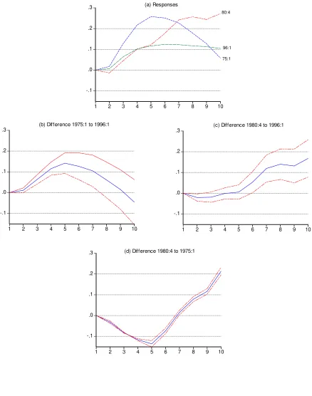
Figures 2a, 3a, and 4a show the impulse response function of unemployment, output, and inflation to an unexpected increase in the Fed funds rate in these dates.18 The other graphs in these figures plot the pairwise differences between responses for some dates along with 90% bootstrap confidence bands. Monetary policy shocks have a strong and lasting negative effect on unemployment during the Volcker period, and the uncertainty around these values increases over the horizon considered. The response of unemployment is also large in the Burns period, but it reaches a peak after five quarters. In the Greenspan period the response of unemployment is substantially smaller than in the previous ones.

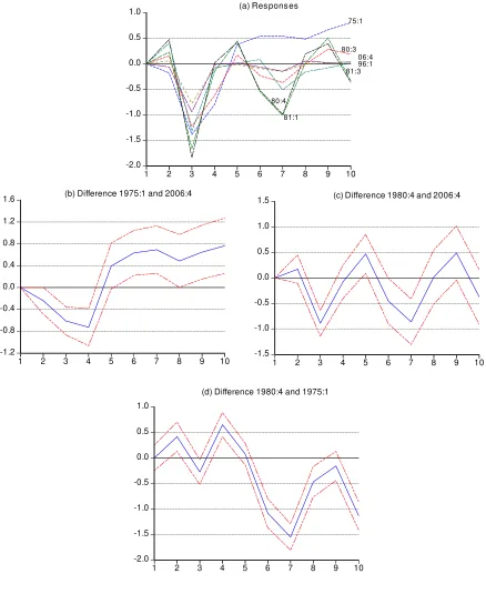
The negative response of output follows a similar pattern, being strongest in the Volcker period, especially between 1980:3 and 1981:3, and weakest in the more recent periods in 1996:1 and in 2006:4. The pairwise differences across dates are substantial and significant when taking into account the 90% bootstrap confidence bands.19 The response of inflation to monetary policy shocks shows an even greater time variation. The largest negative response occurs in the 1975:1, in the Burns period, followed by milder but still negative impact in the Greenspan and the Bernanke periods (1996:1 and 2006:4). On the other hand, inflation shows a positive response in the Volcker period between 1980:4 and 1981:3, even though the VAR considered includes commodity inflation.20

18_{The response of unemployment between 1980:4 and 1981:3 is similar, so we only plot one of these subsamples.}

19_{There is a small but insignificant positive increase in output in the second period for some dates, which is also found by several} authors and is named ‘output puzzle’ (see e.g. Boivin and Gianonni 2002 or Giordani 2004).

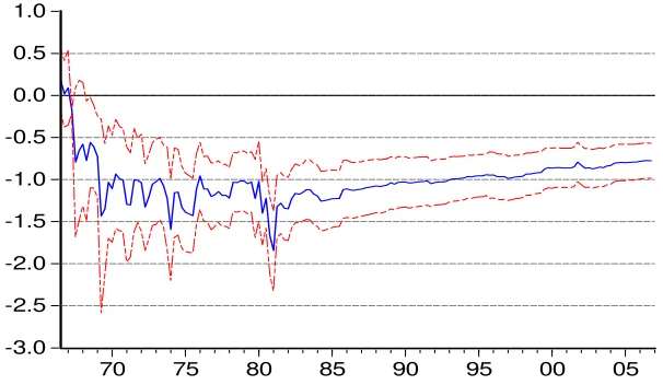
A broader picture of the changes can be seen in the evolution of the impulse response functions over recursive real time samples. As an illustration, Figure 5 plots the time series of the real time response of output to monetary policy shocks in the third quarter, which is the period with strongest response as found in Figure 3a. The response gradually increases (in absolute value) from the beginning of the sample until it reaches a peak in 1981. In fact, the largest responses are found between 1980 and 1982. From then on the response is much more stable and decreases gradually until the end of the sample to values smaller than in the 1970s and 1980s.

Figure 6 shows the evolution of the response of inflation to monetary policy shocks in horizons three and four. The third quarter captures the dynamics of the price puzzle. Some authors have shown that the price puzzle is sensitive to the sample used, and that it is stronger for the period pre-1980 than for post-1980.21 We find that a significant price puzzle is present in only a small part of the sample, between 1977 and 1981, with a sharp decrease in the positive response of inflation in the first quarter of 1981. This suggests that analyses based on comparison of sub-samples can be quite misleading depending on the dates chosen. 22

The dynamics of the response in quarter four plotted in Figure 6 indicates that inflation had the strongest negative response to monetary shocks between 1974 and 1976 (see Figure 4a). The point estimates of the response become positive during the Volcker disinflationary period, and turn negative again from the mid-1980s on. However, the uncertainty surrounding the estimates as shown by the confidence bands only allows concluding that there was large negative response in the mid 1970s compared to other times, and also a significant milder negative response since the mid 1990s and on.

In summary, the evidence confirms previous discussions regarding a recent reduced impact of monetary policy shocks on output, unemployment, and inflation compared to historical values. However, we find that the responses are not only time-varying, but also highly nonlinear with more oscillations in the first part of the sample and more stability in the second part. In addition, there have been some abrupt changes in the responses of inflation to policy shocks.

5.3 Real Time Changes in Systematic Monetary Policy

We consider the evolution of the real time response of interest rate to inflation and unemployment by estimating a forward-looking Taylor rule based on Clarida, Gali, and Gertler (2000):

,

1 3 ,

2 ,

1

0 t tt t tt t t

t

β

β

E

β

E

u

β

i

η

i

u

+

+

+

+

=

π

_{+ςπ +ς −} (12)

21_{See, for example, Balke and Emery (1994), Giordani (2004), Hanson (2004), Castelnuovo and Surico (2006), etc.} 22 _{A counterpart}

where

i

_tis the short term interest rate,

π

_t,t+ςπand

u

t t

u

_,+ς are average inflation and average unemployment from

t

to

t

+

ς

_π, and from

t

to

t

+

ς

_u, respectively. The Taylor principle implies that the long run interest rate response to inflation is:

.

β

β

β

LR

3 1

1

−

=

This parameter is generally interpreted in the literature as a measure of the degree of activism of the systematic monetary policy. If

β

LR

≥

1

,

then the policy rule is said to be activist, that is, there is a more than proportional increase in the nominal interest rate when inflation rises, leading to an increase in the real interest rate. In a passive policy, the increase in the nominal interest rate is less than proportional, which can be measured by

β

LR

<

1

.

Boivin (2006), Primiceri (2005), and Cogley and Sargent (2005) also consider a time-varying degree of activism, and we compare our results to theirs. We follow Cogley and Sargent (2005) in estimating the parameters of the policy rule as projection coefficients from the VAR in two steps. First, the forecasts of average inflation and unemployment are projected onto a set of instruments. The instruments are the forecasts

E

_t−1

π

_t,t+ςπand

u

t t t

u

E

_{−1 ,+ς} for

E

_t

π

_t,t+ςπ and

u

t t t

u

E

_,+ς , respectively, which are obtained from estimating over recursive real time samples the identified VAR.23 In a second step, Equation (12) is estimated with these fitted values, using the nonparametric local least squares method described in Section 3.1. Thus, we do not impose a parametric density for estimating the Taylor rule.

Figure 7 shows the time varying real time estimates of

β

LR

.

The movements broadly agree with the results of several authors, including Judd and Rudebusch (1998), Clarida, Gali, and Gertler (2000), Boivin (2006), and Cogley and Sargent (2001, 2005), which find that the policy rule was passive during the Burns period, and activist during Volcker’s disinflation period and during Greenspan’s chairmanship. However, we find that the uncovered behavior of the parameter is more complex than these general conclusions suggest. The degree of activism displays sharp movements and nonlinearities over time. In particular, the early 1970s are characterized by strong activist policy, which lasted until around the oil shock and recession in 1973-1974. In 1975 the response to inflation falls sharply below one. Policy remains passive until around 1978-1979. During the Volcker disinflation period the degree of activism increases above one and it remains active throughout the rest of the sample. However, notice that

23 _{Similarly to Cogley and Sargent (2005), we project future inflation and unemployment on a constant and two lags of each. In}

addition we assume that

ς

_π= 4 and

ς

_u = 2, consistent with the transmission mechanism of changes in interest rate and the

response of inflation and unemployment. We have also considered other short term horizons such as

ς

_π = 3 and

ς

_u = 3, as

LR

β

falls somewhat in the mid 1980s – but to values still above one, and rises again during the Greenspan period stabilizing around values well above one.

The magnitude of the policy response and its changes over time needs to be evaluated taking into account the statistical uncertainty around these estimates. In fact, there are times in which we can not conclude that the level of the response is below or above one. On the other hand, some changes in the degree of activism are significant when considering the 90% confidence bands, such as a passive policy from the mid to the late 1970s, and an active policy during Volcker’s disinflationary period and during Greenspan’s period.

Compared to the literature, our results are closer to the TVP version of the Taylor rule proposed by Boivin (2006), particularly the specification that allows for three regimes for the variance.24 Using this framework, Boivin (2006) finds variations in the dynamics of the degree of activism at around the same time as ours. Cogley and Sargent’s (2005) results concur with ours in their middle sample, but displays large oscillations in the beginning and end of the sample.25 On the other hand, Primiceri (2005) finds that although policy is more reactive to inflation in the last two decades compared to the 1960s and 1970s, the long run response to inflation remains above one in the entire sample. Primiceri (2005) attributes this difference to the fact that the results are based on smoothed estimates that use full sample information. However, Cogley and Sargent (2005) use a similar framework and estimation methods and find large swings in

β

LR

,

with values reaching below one from the mid to the late 1970s. The difference in timing and magnitude of the changes in the long run response obtained by these papers might be a product of the parametric assumptions made in these models. If the assumptions do not hold, the parameters might be biased and inconsistent. A particular appeal of recursively estimating the proposed model allows detection of discrete local deviations as well as more gradual ones, without smoothing the timing or magnitude of the changes.

5.4

Robustness

Comparison of Results with Alternative Specifications

Results from VAR models are known to be sensitive to their specification. Our standard specification delivers sensible response functions, some of the results being broadly consistent with existing literature. For instance, Bernanke and Mihov (1998), Clarida, Gali, and Gertler (2000), Barth and Ramey (2001), Cogley and Sargent (2001, 2005), Boivin and Gianoni (2002, 2006), Boivin (2006), among others report a similar reduction in the effect of policy shocks on inflation, output (or unemployment). In particular,

24 _{The middle one is from the fourth quarter of 1979 to the fourth quarter of 1982.}

Bernanke and Mihov (1998) use a more sophisticated representation of the Fed’s operating procedure while Barth and Ramey (2001) use long-run restrictions and attain similar findings.

We have also estimated two structural VARs that include three or five variables as discussed in Section 2. The inclusion or exclusion of information in our VAR does not affect the main conclusions obtained. In fact, the results are striking similar. One difference is that, as expected, the exclusion of commodity inflation accentuates the price puzzle – it is significant for a much longer period.26

Next we address the question on whether the results are sensitive to the VAR ordering. Although, this assumption is more appropriate when using revised data, we have alternatively estimated the model assuming that policymakers do not observe contemporaneously the non-policy variables, which is motivated by lags in the collection of data (i.e. ordering the federal funds rate first). We find the results qualitatively equivalent in both cases. There are only minor changes in the size of the innovation variance of the federal funds rate but with the same broad pattern of evolution over time. In addition, we find a larger but insignificant output puzzle when the policy variable is ordered first. This is consistent with the comparison of these orderings in Christiano, Eichenbaum, and Evans (1999). Finally, changing the order of the non-policy variables has insignificant effects on the results.

In summary, the main empirical features that we aim to explain, namely the time-varying changes and reduced effect of monetary shocks on output and inflation, the pattern of changes in variances over time, and time variations in the degree of activism are corroborated by different specifications and identifying assumptions.

We have also estimated recursively a parametric counterpart of the structural VARs with three and five variables and the same identification restrictions as our benchmark specifications. In order to capture heteroskedasticity we estimate the model assuming three different regimes from the variance. The middle one corresponds to the high volatile period between 1979:4 and 1984:1. Based on the variance plotted in Figure 1a, this division captures major heteroskedastic episodes in the monetary policy shocks.27

Comparing the results, we find analogous temporal evolution in the recursive coefficients and variances of shocks obtained with the parametric VAR. Although the patterns are similar, the parametric VAR yields estimates that substantially underestimate or overestimate the nonparametric estimates. As an illustration, Figure 8 compares the dynamics of the variance of interest shocks. The parametric VAR underestimates the variance of interest shocks for most of the sample, except for the period between 1981

26 _{For sake of brevity we do not report the results of the VAR with three variables here. The full range of results for this} specification is reported in a previous version of this paper and is available from the authors on request. We have also estimated this version of the VAR considering changes instead of the level of interest rates as in Gali (1992).

and 1986, when the variance is overestimated.28 If the normality or functional form assumptions on the parametric specification do not hold, the coefficients of the parametric VAR may be biased.

We examine normality of the structural innovations of the parametric structural VAR using several tests.29 Since the innovations are assumed to be serially uncorrelated, we first apply multivariate extensions of the traditional Jarque-Bera test and Kolmogorov–Smirnov (KS) tests.30 The tests are applied to several dates in the sample. For all sub-periods examined we reject the joint normality of innovations with a p-value near zero, even for periods that exclude the highly volatile Volcker’s disinflation period, and for the more recent period. The tests also reject normality equation by equation for all sub-periods considered for at least three equations. Finally, normality is also rejected for the unemployment equation in all sub-samples examined.

We further investigate the normality assumption using Fan, Li, and Min’s (2006) extension of Zheng’s (2000) nonparametric conditional normality test. The statistic critical values are obtained following the bootstrapping procedure suggested by Fan et al (2006) to better approximate their finite-sample null distribution. The test is applied to several sub-periods and to the full finite-sample and we find that it overwhelmingly rejects the assumption of normality at any conventional significance level.

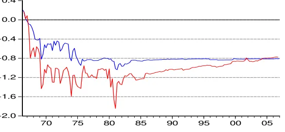
Finally we compare the results of recursively estimating the proposed monetary VAR using only data available in the 2007:1 vintage. This comparison can shed light on differences in findings due to the use of real time versus revised data. As an illustration, we show the difference in the response of output to the identified monetary shock.31 Figure 9 plots the evolution of the response of output in period 3 from the nonparametric VAR estimated over real time recursive samples (same time series as in Figure 5) and the counterpart estimated series obtained using revised data (i.e. each point is the result of estimating the VAR for increasing samples from 1959:1 to 2006:4 using the same dataset as of 2007:1). Although the response shows the same general temporal pattern, the revised version underestimates the negative response of output to interest rate until the 2000s. This is especially accentuated during the Volcker disinflationary period. In addition, the decrease in the impact of monetary policy shock on output in the later part of the sample is much more pronounced when using real time data.

The estimation using revised data also overestimates or underestimates the other parameters of the model during some periods, concealing the impact of shocks that took place in real time. The findings support Orphanides (2001, 2002, 2004), which argue that evidence based on revised data does not

28_{The response of the economy also shows different timing and intensity to interest rate shocks estimated from the parametric} VAR.

29_{We estimate the parametric model with lags}

p=1, 2, 4.

30_{Bai and Ng (2005) propose a method to test for normality on time series data with weakly dependence and apply it to some of} the individual series used in our structural VAR. They find that the normality assumption is rejected for unemployment rate and inflation, but not for output growth.