Maintenance efficient routing in wireless sensor networks

(1)

Maintenance Efficient Routing in Wireless Sensor Networks

Andre Barroso, Utz Roedig and Cormac Sreenan

Mobile & Internet Systems Laboratory, University College Cork, Ireland

Email: {a.barroso u.roedig c.sreenan}@cs.ucc.ie}

Abstract

This paper presents an analysis framework of routing protocols that can be applied to produce sensor fields that are much less expensive to maintain. The framework is based on a maintenance model that is simple, yet flexible enough to capture real world deployment scenarios of sen-sor networks. As an illustration, the framework is used to assess the impact of different forwarding techniques for a known geographical routing protocol on the overall main-tenance costs of different sensor fields. The results obtained indicate that an one-size-fits-all approach for the design of maintenance efficient routing protocols does not hold in large deployments of wireless sensor networks. However, savings of up to 50% in maintenance cost were observed through simple modifications of the forwarding strategy.

1. Introduction

As sensor nodes become cheaper and smaller the domi-nating cost factors of wireless sensor networks will lie in de-ployment and maintenance. Dede-ployment will generally in-volve trained personal and specialized equipment that may include airplanes to drop sensors over areas that cannot be accessed otherwise. Some sensor units may instead require careful placement in the field thus consuming many hours of qualified labor. Furthermore, in long lived systems it is nec-essary to keep the network operational for a period of time that surpasses the lifetime provided by the batteries when the network was first deployed. Maintenance will thus be re-quired and will involve periodic recharging or replacement of batteries in sensor fields that cannot harvest enough en-ergy from the environment to remain operational. The use of large batteries or redundant nodes are solutions that may defer but cannot indefinitely prevent the need for manual intervention. Given the potential high costs, an appropriate design of sensor networks must take deployment and main-tenance needs into consideration.

The frequency of maintenance operations in a sensor field is essentially dependent on the way nodes are

de-pleted. Given the impact of communication in the energy consumption of sensor nodes, the field depletion profile can be greatly influenced by the traffic flow inside the network. Protocols in the network layer can therefore help the shap-ing of favorable depletion profiles accordshap-ing to some appro-priate metric that captures the concept of maintenance effi-ciency.

This paper presents an analysis framework of routing protocols that can be applied to produce sensor fields that are much less expensive to maintain. The framework is based on a maintenance model that is simple, yet flexible enough to capture real world deployment scenarios of sen-sor networks. To the best of our knowledge, this is the first work in the literature to propose a deeper analysis on the costs of deploying and operating wireless sensor networks by way of improving their design.

2. Maintenance in Wireless Sensor Networks

2.1. Concepts and Assumptions

Although the term maintenance may encompass a vast number of different activities, this study adopts the restric-tive definition of a maintenance operation as the replace-ment of batteries from one or more nodes in the sensor field. Human intervention in the field required by equipment dam-age or malfunctioning is intentionally omitted from this def-inition. Since the study aim is the design of protocols able to affect maintenance costs by altering how batteries are de-pleted, sensor nodes are assumed to be reliable. If neces-sary, sensors with limited expected lifetime can be replaced together with batteries.

(2)

2.2. Motivation Scenarios

The problem of maintenance in wireless sensor networks can be better understood by centering on examples of long term deployments where human intervention is periodically needed to keep the field operational. Two such scenarios are presented in the following paragraphs. The scenarios are later used in the discussion of maintenance models.

Precision Agriculture. A promising application of

wire-less sensor networks is in the instrumentation of farming ar-eas to collect data which can be used to enhance crop yields. Crop fields may cover extensive areas and the overlaid sensor network will require periodic battery recharging for continuous operation in situations where energy cannot be extracted from the environment or the extraction is insuffi-cient. The access to individual sensors are likely to be un-problematic as crops are laid for easy reaping. Nevertheless, sensors may be spread over large areas and great distances might be covered to access nodes requiring battery replace-ment.

Habitat Monitoring. Wireless sensor networks have

also been deployed successfully for the monitoring of liv-ing creatures in their habitat. The wireless feature of the technology ensures the system is minimally intrusive.

The structure and characteristics of a sensor field used in habitat monitoring can vary greatly depending on the type of habitat considered. As an example, the monitoring net-work may cover a small area in which sensors are placed in locations with very distinct access requirements. Some sen-sors may be located on the top of trees, others underwater and still other may be on the ground. In each case, the ac-cess to a node requiring battery replacement may involve different equipment, personnel, times and consequently dif-ferent costs.

2.3. Maintenance Model

In order to formalize the study of the impact of how bat-tery depletion affects maintenance costs, a model is required that describes when batteries should be replaced and the costs involved in the replacement. In the following para-graphs the policies and cost structure (the cost model) for the maintenance of wireless sensor networks are described. The maintenance policy and cost model define a mainte-nance model for the network. Later, we show how the main-tenance model is used to assess mainmain-tenance aware routing protocols.

Maintenance policy

The specifics of the maintenance operations and their frequency are defined by the maintenance policy. A sim-ple policy might have the following structure:

A maintenance operation is triggered ev-ery time a node has less than 10% of its initial

battery charge remaining. During the mainte-nance operation, the battery of the depleted node is recharged/replaced.

Different policies are possible depending on the particular-ities of the sensor field, resources available and application requirements.

Although battery recharging of a single node per mainte-nance operation might be reasonable under certain circum-stances, several scenarios justify multiple battery replace-ments per maintenance operation. This is specially true in fields where the cost to access the depleted sensor is domi-nant. In these cases, it makes sense to recharge batteries of all nodes in the vicinity of the depleted sensor even though they are not technically considered depleted.

The concept of vicinity is variable from sensor field to sensor field. In the habitat monitoring scenario described in Section 2.2, nodes placed in a same tree could be consid-ered as part of the same vicinity. The same can be said of sensors placed in a same pond. We refer to a group of nodes in the same vicinity as a maintenance zone. More formally:

A maintenance zone is a set of sensor nodesS such that for every pair of sensorss1, s2 ∈ S ,

the cost of accessings2froms1is negligible.

As the definition implies, sensors in a field are primarily grouped into maintenance zones according to the mainte-nance cost model. Indeed, if the access cost to sensors is de-fined by the geometric distance to reach them, then all sen-sors physically close to each other can be grouped into a sin-gle zone. If access costs to sensors are defined entirely by their absolute position in the field then two sensors physi-cally close to each other, one on a tree and the other in a pond, may not belong to the same zone.

In this study, for simplicity, maintenance zones are al-ways a partition of the area covered by the sensor field.

Cost Model

Sensor fields may contain nodes underneath water, on the top of hills or spread over a large flat area. In each of these situations, the equipment, the personnel and the effort necessary to perform a maintenance operation have differ-ent characteristics that will affect the maintenance cost.

The cost of servicing a sensor in a sensor field can be di-vided in many different ways. It suffices for the purpose of this study to decompose the total cost in two factors:

• Access Cost : one-time resources spent while access-ing the sensor to be serviced.

(3)

These cost components are added to produce the mainte-nance costCm(s)of servicing a single nodesin the sensor

field:

Cm(s) =Access Cost+Recharging Cost (1)

A concrete example of a cost model helps the under-standing of the concepts just presented. Consider the de-ployment of wireless sensor nodes for environmental moni-toring in redwood trees at University of California Botanical Garden’s Mather Redwood Grove [10]. In this deployment, several sensor nodes are attached in different positions of trees that can be hundreds of feet tall. Climbing equipment is used to deploy such sensors. The access cost to reach an individual node may include the vehicle/fuel used to reach the sensor field and the labor cost of the people involved. Such costs are proportional to the distances involved and the difficulty involved in climbing the trees. Once the sen-sors are reached, the recharging cost involves the batteries replaced.

2.4. Applying the Maintenance Model

The model previously defined can be used to quantify the total cost of maintaining a sensor field. Indeed, every main-tenance operation incurs a cost defined by equation 1. Dur-ing the lifetime of a sensor field,Imaintenance operations will take place. The total maintenance costCtof the

sen-sor field, maintained according with policyP, is then given by:

Ct(P) = I X

i=0

Cmi (2)

This cost can be improved by reducing eitherCm orI.

Reduction ofCm cannot be achieved by altering the

pro-file of battery depletion in the sensor field. The value of this parameter is dependent on elements such as transportation costs, labor costs, etc. Therefore, the goal of reducing to-tal maintenance cost by minimizingCmis out of the scope

of this study. Reduction ofI, however, can be achieved by a combination of factors including the choice of mainte-nance policy, design and operation of sensor networks as discussed next.

2.5. Towards Maintenance Efficiency in Wireless

Sensor Networks

A maintenance policy impacts total maintenance costs of a sensor field by affecting the frequency in which nodes are recharged. As mentioned in Section 2.3, sensor fields where the cost of a maintenance operation is solely defined by the access cost should opt for a policy in which nodes in

the same maintenance zone are replaced concurrently. This procedure reduces the frequencyIof operations in the field without adding any extra cost (the only cost is incurred in accessing the zone).

The consequence of adopting the strategy of recharging the battery of several nodes at a single access cost is the possible presence of nodes in a zone that are far away from depletion when recharged. From the perspective of a sys-tem designer, this situation means that individual nance zones unequally depleted at the moment of mainte-nance contain energy that should have been used to delay the maintenance operation, increase the reliability of com-munication or any other use. The energy was “wasted” since using it would bring benefits without incurring additional costs.

A system designer affects the maintenance cost by choosing to deplete the sensor field in accordance with a profile that shapes not only the number I of mainte-nance operations but also where these operations take place in the case of sensor fields where different zones in-cur different access costs. Some level of load balanc-ing should be applied for uniform depletion of the sensor field as a whole and across the zones. On the other hand, de-pletion should take place more slowly in zones with high access costs.

Finally, maintenance costs are affected by the way appli-cations use the network. As an example, an application may operate different sections of the network more intensely at given periods while other applications may continuously operate the field in a uniform way.

3. Maintenance Efficient Routing Protocols

Routing protocols hold a great potential for affecting maintenance costs since battery depletion can be shaped at a network level by controlling the flow path of packets. This section deals with the process of evaluating and designing routing protocols that try to incorporate maintenance effi-ciency in the system. The first step in this process is the def-inition of an appropriate metric able to capture this concept. Variations of a geographical routing protocol are used to ex-emplify evaluation and design for maintenance efficiency.

3.1. Maintenance Metrics

(4)

nonethe-Zone B

[image:4.612.324.552.73.181.2]

Access cost origin point Zone A

Figure 1. Maintenance metric for precision agriculture scenario

less inappropriate for the design of maintenance efficient sensor networks since they oversimplify maintenance costs. Energy efficiency overstates the importance of energy con-sumed in the system by ignoring the fact that the cost of the Joules injected into batteries may be irrelevant to the over-all maintenance cost. Maximizing network lifetime is an ob-jective more aligned with the problem of achieving mainte-nance efficiency. However, it also neglects the costs differ-ences of depleting the sensor field in different areas.

A suitable metric for the performance assessment of maintenance efficient routing protocols can be derived di-rectly from the maintenance model presented in Section 2.3 in the form condensed by equation 2. The problem of in-stantiating a metric for a particular system requires knowl-edge of the maintenance policyPand the appropriate main-tenance operation costs for the field. As an illustration, con-sider the definition of a maintenance metric for routing pro-tocols on the two wireless sensor network scenarios de-scribed in Section 2.2. In both scenarios it is assumed a pol-icyP that replaces nodes of an entire maintenance zone in each operation. Furthermore, the recharging cost is consid-ered negligible.

Precision Agriculture Scenario. The sensor field is

par-titioned in artificial zones for maintenance purposes as de-picted in Figure 2. Since recharging costs are assumed neg-ligible, the maintenance operation cost is defined by the ac-cess costs to each zone. The crop field is assumed to cover an extensive area and the access to individual zones is un-problematic. Therefore the access cost can be characterized solely by the euclidean distance from the zone to a geo-graphical point where the personnel involved in the main-tenance starts their journey (all operations are assumed to begin in this point). In the figure, the maintenance cost for nodes in zone B is thus higher than for nodes in zone A.

Habitat Monitoring Scenario. As in the previous

sce-nario, the sensor field is partitioned in artificial zones and maintenance operation cost is defined by the access costs to each zone. The field is assumed to cover a small area and zones lie in very different terrains. In Figure 2, the

Zone B

Zone A Lake

Figure 2. Maintenance metric for habitat mon-itoring scenario

nance cost for nodes in zone A is higher than for nodes in zone B since the former contain nodes in a lake.

3.2. Design of Maintenance Efficient Routing

Pro-tocols

The maintenance model and respective metric constitute the starting point in the process of designing routing proto-cols for maintenance efficiency. In this section, variations of a geographical routing protocol are proposed, each explor-ing different aspects of the system and maintenance model. The efficiency of each approach is evaluated in Section 4. The choice of a geographical routing protocol as the ba-sis of this study was based on its flexibility in finding alter-native paths towards the destination when forwarding deci-sions are local. In general, as long as the geographical lo-cation of the destination is known, a path towards it can be found. It is therefore easy to generate variations of routes towards the desired node. Nonetheless, the reasoning pre-sented in the study can be extended to other types of proto-cols, such as directed diffusion[3] and broadcast built trees rooted at the sink. The protocol variations presented next explore only the design space of packet forwarding based only on local information. No attempt is made to achieve global optimality on the solutions given the cost of obtain-ing the needed data in large scale networks.

GPSR. The Greedy Perimeter Stateless Routing (GPSR)

protocol is a well known geographic routing protocol de-scribed in [5]. All nodes in GPSR must be aware of their position within a sensor field. Each node communicates its current position periodically to its neighbors through bea-con packets. Upon receiving a data packet, a node analyzes its geographic destination. If possible, the node always for-wards the packet to the neighbor geographically closest to the packet destination. If there is no neighbour geograph-ically closer to the destination, the protocol tries to route around the “hole” in the sensor field.

GPSR-R. A GPSR variation in which a packet is

[image:4.612.60.278.73.179.2]

(5)

operations in the sensor field by load balancing the traffic in the network.

GPSR-ME. Packets are forwarded to the

neigh-bour node closer to the destination with the maximum battery energy level. This approach seeks to reduce the fre-quency of maintenance operations in the sensor field through a guided load balancing as opposed to the ran-dom approach of GPSR-R.

GPSR-MZ. Messages are forwarded to a neighbour

node closer to the destination within a maintenance zone of minimum cost among the candidates. In case multiple can-didates exist conforming to this criteria, one of them is cho-sen randomly. The approach tries to reduce the total cost of maintenance by avoiding expensive zones.

GPSR-MZME. Messages are forwarded to a neighbour

node closer to the destination within a maintenance zone of minimum cost among the candidates. In case multiple can-didates exist conforming to this criteria, the one with maxi-mum remaining energy is chosen. The approach tries to re-duce the total cost of maintenance by avoiding expensive zones. As a subordinate goal, the approach seeks to reduce the frequency of maintenance operations in the sensor field by load balancing the traffic in the network.

GPSR-MEMZ. Messages are forwarded to a neighbour

node closer to the destination with the maximum battery en-ergy level. In case multiple candidates exist conforming to this criteria, the one within a maintenance zone of minimum cost among the candidates is chosen. The approach tries to reduce the frequency of maintenance operations in the sen-sor field through load balancing. As a subordinate goal, the approach seeks to reduce the total cost of maintenance by avoiding expensive zones.

4. Evaluation

4.1. Experiment Setup

A comparative analysis of the merits of each variation of the geographical routing protocol was conducted through simulations in the precision agriculture and habitat moni-toring scenarios presented in Section 2.2. In each scenario, the goal is to understand the impact of different forward-ing criteria in the overall maintenance cost and energy con-sumption of a long-lived battery powered system. A detailed characterization of the experiment is presented next.

Simulator. For the experiments, a lightweight

event-driven simulator was written in C++. Its main design objec-tives were simplicity and scalability with the size of the net-work. Given the level of abstraction required in this study, the option for a fast tool over more complex simulators such as ns-2 is justifiable. A node is able to transmit/receive packets to other nodes inside a well defined transmission range and each node incorporates a battery with a

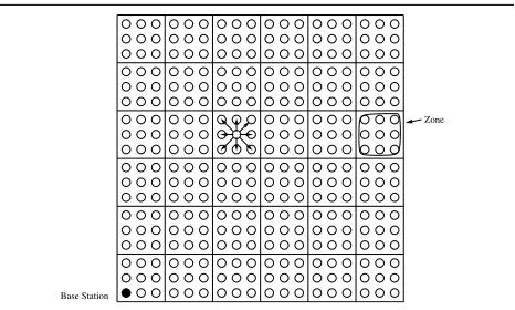
maxi-Zone

[image:5.612.321.554.73.213.2]

Base Station

Figure 3. Sensor field structure for the exper-iment

mum energy capacity. The energy level of a battery is re-duced by a fixed amount with every packet transmitted. The access to the shared media is collision-free.

Sensor Field. The sensor field is a grid of wireless sensor

nodes organized as depicted in Fig. 3. All sensors have the same specification and are equally spaced from each other. A full battery allows for 1000 packet transmissions. Mainte-nance zones were dimensioned to be much smaller than the total number of nodes in the field number. The grid is com-prised of 324 nodes organized in a 18x18 arrangement and it is partitioned in 36 zones, each including 9 nodes. The ra-dio range is adjusted so that only immediate adjacent nodes can communicate (i.e., 8 neighbors or less per node). A base station collecting reports from other sensors in the field is placed at the bottom left-most corned of the grid.

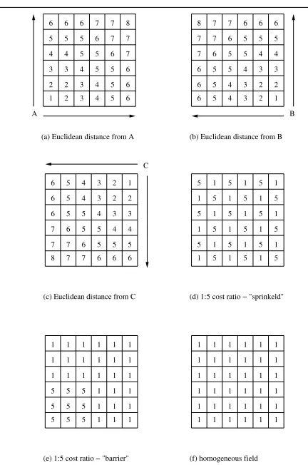
Maintenance Model. In both scenarios analyzed, the

cost model was chosen to reflect the assumption that access costs will dominate the total maintenance cost of the sen-sor network. The maintenance policy is such that a main-tenance operation is triggered every time a node has less than 10% of its initial battery charge remaining. During the maintenance operation, the batteries of ALL nodes in the same zone are recharged/replaced.

(6)

af-6 6 6 7 7 8

5 5 5 6 7 7

4 4 5 5 6 7

3 3 4 5 5 6

2 2 3 4 5 6

1 2 3 4 5 6

A

(a) Euclidean distance from A

8 7 7 6 6 6

7 6 5 5 5

7 6 5 5 4 4

6 5 5 4 3 3

6 5 4 3 2 2

6 5 4 3 2

(b) Euclidean distance from B 7

B

6 5 4 3 2 1

6 5 4 3 2 2

6 5 5 4 3 3

7 6 5 5 4 4

7 7 6 5 5 5

8 7 7 6 6 6

(c) Euclidean distance from C

1

C

1 1 1 1 1 1

5 5 5 1 1 1

(e) 1:5 cost ratio − "barrier"

5 1 5 1 5 1

1 5 1 5 1 5

5 1 5 1 5 1

1 5 1 5 1 5

5 1 5 1 5 1

1 5 1 5 1 5

(d) 1:5 cost ratio − "sprinkeld"

[image:6.612.62.278.70.396.2]

(f) homogeneous field

Figure 4. Access costs for simulated scenar-ios

fected by such variation.

Operation Model. It is assumed that, at any time,

ex-actly one sensor is actively sending data to the base-station. This sensor is selected randomly within the sensor field. A node sendsnmessages before a new node is selected. Each message sent is separated from the previous one by an in-terval of 5 seconds. In this setup, the network generates the same number of data packets per unit of time for every run of the simulator.

4.2. Comparative Evaluation

The different forwarding criteria described in 3.2 are compared according to the following metrics:

• Total Maintenance Cost, computed as defined in eq. 2;

• Total Number of Zone Accesses;

• Total Dissipated Energy;

• Average Number of Hops defined as the ratio between the sum of hops traveled by each report message

gen-erated in the field and the total number of report mes-sages.

The total maintenance cost indicates the impact of the for-warding technique on the actual cost of maintaining the sen-sor field. The total number of zone accesses indicates the frequency of accesses to maintenance zones during the ex-periment. For two protocols with similar maintenance costs, this metric reveals whether many low access cost or a few high access cost zones were depleted. The total dissipated energy indicates the number of Joules injected in the sys-tem. Finally, the average number of hops exposes the po-tential impact of the forwarding techniques on latency.

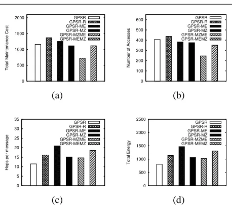
Experiment 1 - Precision Agriculture Scenario In the

first experiment, routing protocols are simulated in fields where zone access costs are proportional to the euclidean distance of a single geographical point. Figure 5 shows the results for a field where the reference geographical point for computing costs coincides with the base station location (see fig. 4(a)). The field is operated in a way that each node sends a single message before a new node is randomly se-lected to report (i.e.,n= 1).

(7)

0 500 1000 1500 2000

Total Maintenance Cost

GPSR GPSR-R GPSR-ME GPSR-MZ GPSR-MZME GPSR-MEMZ

0 100 200 300 400 500 600

Number of Accesses

(a) (b)

0 5 10 15 20 25 30 35

Hops per message

0 500 1000 1500 2000 2500

Total Energy

[image:7.612.62.291.71.275.2]

(c) (d)

Figure 5. Simulation results for sensor field

of fig. 4(a) andn= 1

As a final remark, note that the most energy efficient scheme according to fig. 5(d) is GPSR, but this fact does not directly translates into maintenance efficiency as can be seen in fig. 5(a).

Impact of Euclidean Distance Reference. The

perfor-mance of GPSR-MZME and GPSR-MZ in fields where zone access costs are proportional to the euclidean distance of a single geographical point is greatly dependent on the relative position of this point and the base-station. In situa-tions where the reference geographical point and the base-station are approximately in the same direction, the goals of minimizing maintenance costs and delivering a packet to the destination are aligned. Indeed, forwarding packets to zones of minimum costs also means approaching the base-station. This synergy contributes to energy savings in the field since the path traveled by messages tend to be shorter. In scenar-ios where the base-station and reference geographical point are not in the same direction a conflict arises in the forward-ing process. The effort of maintainforward-ing packets in zones of low access cost hinders the movement towards the base sta-tion resulting in longer paths. As a consequence of this con-flict, GPSR-MZME and GPSR-MZ perform worse than the other forwarding approaches where zone access costs are not taken into consideration or are only subsidiary in the forwarding decision process. Figure 6 shows the total main-tenance cost of the sensor field when the geographical refer-ence point is respectively located at corners B and C of the sensor field (see fig 4). The graphs indicate the poor perfor-mance of GPSR-MZME and GPSR-MZ in comparison to the other techniques.

0 1000 2000 3000 4000 5000

0 1000 2000 3000 4000 5000 6000 7000

(a) Euclidean dist. from B (b) Euclidean dist. from C

Figure 6. Total maintenance cost when base-station and euclidean distance reference are in different locations

Impact of Operation Dynamics. In the simulation,

pa-rameterndescribed in 4.1 controls the operation dynamics of the network. Whenn= 1, there is no correlation between the origin of two consecutive messages generated in the sen-sor field. Each message is generated at a random node and forwarded to the base-station according to a chosen scheme. As the value ofnincreases, the behaviour of the traffic as-sumes a hot-spot profile where traffic is originated from a sole location for extended periods of time before moving to a different point in the network. The impact of this pa-rameter is specially noticeable in the comparative perfor-mance of GPSR with the other techniques. When the value of nis high, consecutive messages generated at the same node and forwarded through GPSR will follow always the same path. This behaviour causes the fast depletion of nodes along this path and an increase of the number of mainte-nance operations required. Whennis low, this negative ef-fect is counter-balanced by the randomization of the packet sources. This randomization creates a form of load balanc-ing in the field that is independent of the forwardbalanc-ing tech-nique. Other techniques already incorporate load balancing schemes and therefore are less affected than GPSR. Figure 7 depicts the total maintenance cost of the forwarding tech-niques whenn = 100. Compare the values obtained with those shown in figure 5 wheren= 1. GPSR performance is greatly reduced by the absence of randomization in the se-lection of forwarding paths with the higher value ofn.

Experiment 2 - Habitat Monitoring Scenario In the

[image:7.612.320.552.75.170.2]

(8)

0 500 1000 1500 2000 2500 3000

Figure 7. Total maintenance cost for sensor

field of fig. 4(a) andn= 100

0 500 1000 1500 2000

0 200 400 600 800 1000

Number of Accesses

(a) (b)

Figure 8. Simulation results for sensor field

of fig.4(d) andn= 1

MZ and GPSR-MZME are respectively 65% and 55% of the cost incurred by GPSR. Nonetheless, the overall num-ber of maintenance accesses to the field are highest when these techniques are applied (figure 8(b)). This result oc-curs because bypassing expensive zones reduces the num-ber of alternative routes in the fields creating hot spot points that deplete faster and require battery replacement more of-ten. As expected, the same phenomena occurs in the sen-sor field configuration of figure 4(e). However, because ex-pensive zones cannot be really bypassed, GPSR-MZ and GPSR-MZME do not perform as well as in the previous case as shown in figure 9. In both scenarios, the perfor-mance of GPSR-MZ and GPSR-MZME relative to the other techniques is very dependent on the cost ratio between the expensive and inexpensive zones. In general, the higher the ratio, the better the relative performance. On the other hand, if this ratio is close to one, then these protocols will under perform all the others since they require more ac-cesses to the field. The simulation result when all zones have the same access cost is shown in figure 10. Note that in this case, MZ degenerates into R and GPSR-MZME degenerates into GPSR-ME. It is also worth men-tioning that in this scenario, the objective of maximizing the network lifetime (defined as the time to first depletion) co-incides with the objective of minimizing maintenance costs.

0 500 1000 1500 2000 2500

field of fig. 4(e) andn= 1

200 250 300 350 400 450 500 550 600 650

[image:8.612.61.293.235.334.2]

field of fig. 4(f) andn= 1

5. Related work

Research related to maintenance in wireless sensor net-works has been generally restricted to the development of remote network reprogramming schemes and energy-efficient hardware/software. Tools allowing remote network programming have received special attention in recent years because of the recognition of the difficulties associated with accessing large number of nodes deployed in possibly hos-tile environments. Schemes such as Deluge[2] and Maté[6] were thus proposed to disseminate code in wireless sensor networks without human intervention.

Regarding the development of operational software for such networks, the focus has been on the extension of the lifetime of the system through the use of techniques that conserve batteries as much as possible. Several data dis-semination protocols were designed to meet this objective. In [1], a flow augmentation algorithm is proposed to de-fine paths that maximize the system lifetime in ad-hoc net-works, where lifetime is defined as the length of time un-til the first battery drain-out among all nodes. The authors in [7] use a variation of this metric and develop an approx-imation algorithm calledmax−min zPmin to solve the

(9)

Sensor networks can be powered primarily or secondar-ily by extracting energy from the environment [4]. This mechanism is known as energy scavenging or harvesting. Although energy scavenging is a promising technique in many applications for wireless sensor networks, there will be deployments where the only form of energy available is battery provided or the harvested energy is insufficient to cover the energy budget. In these scenarios, the need for pe-riodic battery recharging will still exist for long term sys-tems. To our knowledge, this is the first work in the litera-ture to propose a deeper analysis of the costs of deploying and operating wireless sensor networks with means for im-proving their design.

6. Conclusions

Although energy efficiency is an essential aspect for the practical deployment of large scale wireless sensor net-works, this attribute represents only one aspect of a multi-dimensional problem. Clearly, by solely extending the life-time of batteries it is possible to extend the lifelife-time of a sys-tem, all other conditions being equal. This approach how-ever does not address the cost of recharging individual bat-teries. As a consequence, systems that require less mainte-nance interventions may incur higher costs in practice. Fur-thermore, this approach largely ignores the effects of “re-pairing” the system after depletion. Indeed, different main-tenance policies will affect the way batteries can be depleted in the system while preserving low costs. A group of batter-ies assigned to always be replaced together is for instance maintained at the rate of its fastest depleting node. In such a case, other nodes in this group can speed up their de-pletion rate without affecting the maintenance cost of the group. Nodes can use this “free” energy for different pur-poses, such as increased fault-tolerance or quality of ser-vice.

The experiments conducted in this study demonstrated that an one-size-fits-all approach for the design of mainte-nance efficient routing protocols does not hold in large de-ployments of wireless sensor networks. The variability of scenarios makes it impossible for a single technique to per-form consistently well. Indeed, applying techniques that ex-plicitly take into consideration the cost of accessing certain zones in the field might be counterproductive in scenarios where the objective of minimizing such costs is entirely at odds with the objective of delivering packets to their desti-nation. This observation benefits protocol designer as much as the architect of the sensor field which should make sure conflict of objectives are minimized (for instance, through a proper placement of the base station). In the general case, the model and analysis technique introduced in this paper can be applied to produce fields that are much less expen-sive to operate. In the experiments conducted, savings of up

to 50% in maintenance cost were observed in the long run.

Acknowledgments

The support of the Informatics Research Initiative of En-terprise Ireland is gratefully acknowledged.

References

[1] J.-H. Chang and L. Tassiulas. Energy Conserving Routing in Wireless Ad-Hoc Networks. In INFOCOM 2000. Nine-teenth Annual Joint Conference of the IEEE Computer and Communications Societies, volume 1, pages 22–31, 2000. [2] J. W. Hui and D. Culler. The Dynamic Behavior of a Data

Dissemination Protocol for Network Programming at Scale. In SenSys ’04: Proceedings of the 2nd international confer-ence on Embedded networked sensor systems, pages 81–94. ACM Press, 2004.

[3] C. Intanagonwiwat, R. Govindan, D. Estrin, J. Heidemann, and F. Silva. Directed Diffusion for Wireless Sensor Net-working. Networking, IEEE/ACM Transactions on, 11(1):2– 16, Feb 2003.

[4] A. Kansal and M. B. Srivastava. An Environmental Energy Harvesting Framework for Sensor Networks. In Proceedings of the 2003 international symposium on Low power electron-ics and design, pages 481–486. ACM Press, 2003.

[5] B. Karp and H. T. Kung. GPSR : Greedy Perimeter Stateless Routing for Wireless Networks. In Mobile Computing and Networking, pages 243–254, 2000.

[6] P. Levis and D. Culler. Maté: A Tiny Virtual Machine for Sensor Networks. In ASPLOS-X: Proceedings of the 10th international conference on Architectural support for pro-gramming languages and operating systems, pages 85–95. ACM Press, 2002.

[7] Q. Li, J. Aslam, and D. Rus. Hierarchical Power-Aware Routing in Sensor Networks. In DIMACS Workshop on Per-vasive Networking, Rutgers University, May 2001.

[8] S. Lindsey and C. Raghavendra. PEGASIS: Power-Efficient gathering in sensor information systems. In IEEE Aerospace Conference, volume 3, pages 3–1125 – 3–1130. IEEE, 2002. [9] A. Manjeshwar and D. P. Agrawal. TEEN: A Routing Proto-col for Enhanced Efficiency in Wireless Sensor Networks. In Proceedings of the 15th International Parallel & Distributed Processing Symposium, page 189. IEEE Computer Society, 2001.

[10] S. Yang. Redwoods go high tech. UC Bekeley News, July 2003. Press Release.