Munich Personal RePEc Archive
Hyper-spherical and Elliptical Stochastic
Cycles
Luati, Alessandra and Proietti, Tommaso
Department of Statistics - University of Bologna, SEFEMEQ,
University of Rome "Tor Vergata"
11 May 2009
Online at
https://mpra.ub.uni-muenchen.de/15169/
Hyper-spherical and Elliptical Stochastic Cycles
Alessandra Luati Department of Statistics
University of Bologna
Tommaso Proietti S.E.F. e ME. Q.
University of Rome “Tor Vergata”
Abstract
A univariate first order stochastic cycle can be represented as an element of a bivariate first order vector autoregressive process, or VAR(1), where the transition matrix is associated with a Givens rotation. From the geometrical viewpoint, the kernel of the cyclical dynamics is described by a clockwise rotation along a circle in the plane. The reduced form of the cycle is either ARMA(2,1), with complex roots, or AR(1), when the rotation angle equals2kπor(2k+ 1)π, k= 0,1, . . ..
This paper generalizes this representation in two directions. According to the first, the cyclical dynamics originate from the motion of a point along an ellipse. The reduced form is also ARMA(2,1), but the model can account for certain types of asymmetries. The second deals with the multivariate case: the cyclical dynamics result from the projection along one of the coordinate axis of a point moving inRn
along an hyper-sphere. This is described by a VAR(1) process whose transition matrix is obtained by a sequence ofn-dimensional Givens rotations. The reduced form of an element of the system is shown to be ARMA(n,n−1). The properties of the resulting models are analyzed in the frequency domain, and we show that this generalization can account for a multimodal spectral density.
The illustrations show that the proposed generalizations can be fitted successfully to some well-known case studies of the econometric and time series literature. For instance, the elliptical model provides a parsimonious but effective representation of the mink-muskrat interaction. The hyper-spherical model provides an interesting re-interpretation of the cycle in US Gross Domestic Product quarterly growth and the cycle in the Fortaleza rainfall series.
1
Introduction
Modeling and interpreting cycles has attracted a great deal of attention in the time series literature. Many substantive applications can be found in diverse fields such as macroeconomics, biology, physics,
meteorology and climatology.
Our current paradigm draws from the pioneering work of Yule (1927), who derived a stochastic cycle model by randomly shifting the amplitude and the phase of a deterministic cycle (a sine wave). Yule
showed that this is equivalent to an autoregressive model,ψt= 2 cosωψt−1−ψt−2+ξt, where2π/ω
is the cycle period and ξtis a random source, i.e. a white noise process. Kendall (1945) provides an interesting review of early work on stochastic cycles, and further insight on the impact of this work on econometrics can be gained from Morgan (1990). Nonlinear extension have been provided by Tong and Lim (1980), whereas Gray, Zhang, and Woodward (1989) consider a fractionally integrated extension.
An alternative derivation of a stochastic cycle is based on a two-dimensional vector autoregressive model, describing the path of point on the plane whose position at timetis obtained by rotating coun-terclockwise by an angleωits position at timet−1, and adding a a random perturbation. Damping is
introduced by propagating only a constant proportion of the previous coordinates, so that the skeleton of the dynamic system eventually spirals down to the origin of the coordinate system. This framework is
adopted by Harvey (1989) and West and Harrison (1989, 1997), and produces a marginal ARMA(2,1) process with pseudo-cyclical behavior for each of the two coordinates.
The paper proposes two extensions of the circular stochastic model. The first deals with an elliptical
cycle model, which arises from the trajectory of a point on an ellipse. The second extension generalizes the idea inn > 2 dimensions and obtains the cyclical dynamics from the path of a point on a sphere
or an hyper-sphere. This is achieved via a first order vector autoregressive model with transition matrix resulting from the product of matrices performing Givens rotations in an-dimensional space. We show that the final equations form is ARMA(n, n−1) and we provide a closed form expression for its
spec-tral density. The relevance of these extensions is discussed using three empirical illustrations, the first concerning the estimation of the cyclical component in the growth rate of U.S. gross domestic product.
The second deals with the series of rainfall at a location in Brazil. The third applies the elliptical cycle to model the mink-muskrat interaction.
The paper is organized as follows. Section 2 reviews in details the circular stochastic cycle model.
The elliptical and higher dimensional extensions are developed in sections 3 and 4, respectively. Section 5 presents three main applications. In section 6 we discuss the results.
2
Circular stochastic cycles
A stochastic cycle model can be derived from the recursive representation of a deterministic cycle by a
equa-tion:ψt−2ρcosωψt−1+ρ2ψt−2 = 0, whereω∈[0, π]is the cycle frequency in radians, and introduced
random disturbances on the right hand side, so as to obtain variation in the phase and the amplitude of the fluctuations. The approach taken by Hannan (1964) is to define a (seasonal) cycle as follows:
ψt=αtcosωt+α∗tsinωt,
whereαtandα∗t are uncorrelated first order autoregressive processes; This process yields the variation in the phase and the amplitude of the fluctuations sought by Yule as it clear when it is rewritten as
ψt=Atcos(ωt+ϑt), whereAt= (α2t+αt∗2)1/2is the random amplitude, andϑt= arctan (α∗t/αt)is the random phase in radians.
Harvey (1989) and West and Harrison (1989, 1997) use an alternative formulation, which definesψt as an element of a bivariate vector autoregressive process:
"
ψt
ψt†
#
=ρ
"
cosω sinω
−sinω cosω
# "
ψt−1
ψt†−1
#
+
"
κt
κ†t
#
, (1)
whereκt ∼NID(0, σ2κ)andκ
†
t ∼NID(0, σκ2)are mutually independent error terms,ψ
†
t is an auxiliary process which appears by construction in order to formψt, measured in radians, and ρ ∈ [0,1]is a damping factor. When ρ = 1, the skeleton describes the counterclockwise motion of a point along a
circle inR2.
This model has been applied to macroeconomic time series by Harvey (1985) and Harvey and Jaeger (1993). Various modifications and extensions have been proposed in the literature: see, among others,
Haywood and Tunnicliffe-Wilson (2000), Harvey and Trimbur (2003), Trimbur (2006). The reduced form of (1) is the ARMA(2,1) process
(1−2ρcosωL+ρ2L2)ψt= (1−ρcosωL)κt+ρsinωκ†t−1 (2)
whereLis the lag operator,Lhyt =yt−h. Whenρis strictly less than one the cycle is stationary with E(ψt) = 0, Var(ψt) = σ
2 κ
(1−ρ2), Corr(ψt, ψt−h) = ρhcos(hω), that can be easily calculated, as (1) is a
VAR(1) process (L¨utkepohl, 2006). The power spectrum is given by
f(λ) = σ 2
κ
2π
1 +ρ2−2ρcosωcosλ
1 +ρ4+ 4ρ2cos2ω−4ρ(1 +ρ2) cosωcosλ+ 2ρ2cos(2λ). (3)
Forρthat tends to unity, the spectrum reaches its maximum at a frequencyλthat tends to the frequency
of the cycle,ω. As long asρdecreases, the maximum of the spectrum is attained for values ofλ < ω, as stated in the following proposition, proved in Appendix A.
Proposition 1The maximum of the power spectrum (3) is attained for
λ= arccos
(
1 +ρ2 2ρcosω
Ã
1−sinω
s
1− 4ρ 2
(1 +ρ2)2 cos2ω !)
Henceforth, we shall refer to (1) as a circular stochastic cycle. From a geometrical point of view, the cycle dynamics are obtained clockwise rotation on a plane, around the origin, of the vectorψt−1 = [ψt−1 ψt†−1]′ by the angleω, damped through the factorρ. The rotation is represented by the Givens
matrix
G(ω) =
"
cosω sinω
−sinω cosω
#
. (4)
In fact,G(ω) belongs to the special orthogonal groupSO(2), made of all the orthogonal matrices in
R2 with determinant equal to one, i.e. SO(2) = {G ∈ R2×2,G−1 = G′,det(G) = 1}. Each time the vector ψt−1 is rotated, it is contracted through the factor ρ, so to account for the dampening of the fluctuations, or zero long run persistence. The next two sections will deal with modifications and multivariate extensions of the circular model.
3
Elliptical stochastic cycles
Our first generalization deals with the shape of the cyclical component. In particular, we define the cyclical dynamics from the motion of a point along an ellipse inR2rather than along a circle. According to the orientation of the ellipse, the model will be able to account for a faster or slower transition between
positive and negative states. Letting α > 0, β > 0 be two dilation coefficients, the path of a two-dimensional point that moves counterclockwise along an ellipse is obtained from a deterministic bivariate
difference equation with transition matrix
E(ω) =
"
α 0
0 β
#
G(ω),
whereG(ω)is given in (4). The matrixE(ω)performs the elliptical rotation by an angleω; the dilation coefficients amplify or reduce the two coordinates.
The elliptical stochastic cycle is then defined as
"
ψt
ψt†
#
=E(ω)
"
ψt−1
ψ†t−1
#
+
"
κt
κ†t
#
, (5)
withκt∼NID(0, σ2κI). The reduced form of (5) is the ARMA(2,1) process
(1−(α+β) cosωL+αβL2)ψt= (1−βcosωL)κt+αsinωκ†t−1.
It is immediately clear that the stochastic cycle is stationary ifαβ <1and(α+β) cosω <2. The power spectrum is given by
f(λ) = σ 2
k
2π
1 +α2sin2ω+β2cos2ω−2βcosωcosλ
Whenα=β=ρwe find the first order stochastic cycle (1), with spectrum (3). Ifβ= 1α = cosω1 −tanω, then the autoregressive polynomial has unit roots and the cycle is nonstationary. Note that in this case,
α = cosω1 + tanωandαβ = 1,(α+β) cosω = 2. For this(α, β)pair, if one switches off the shocks, i.eκt = κ†t = 0,∀t, then equation (5) describes the deterministic motion along an ellipse. As a matter of fact, the cartesian coordinates of a point on an ellipse of equation ψ
2 t
α2 +
ψt†2
β2 = 1, and centered at the
origin, areψt = αcos(ωt) andψt† = βsin(ωt), whereω is the angle between the axis α(β) and the auxiliary circle of radius equal toα(β), representing the position of a point moving along the ellipse. The factorsαandβ account for an asymmetric dampening of the fluctuations and eitherαorβ can assume
value equal to one (or greater). Forα, β → 1the spectral power of the cycle (5) is more concentrated near the spectral peak than the cycle (1) whenρ→1.
Proposition 2The maximum of the power spectrum (6) is attained for
λmax = arccos (
1 +R2 2βcosω
Ã
1−sinω
s
1− G
(1 +R2)2 cos2ω !)
,
where R2 = α2sin2ω+β2cos2ω and G = sin12
ω[(1 +R
2)(1 +αβ+ β
α +β2)− β
α((1−αβ)2 +
cos2(ω)(α+β)2)−(1 +R2)2].
Ifα =β =ρ, then(1 +R2) = 1 +ρ2andG= 4ρ2, hence, we find Proposition 1. Furthermore, as
long as eitherαorβare different than one, the maximum of the spectrum is closer toωforβ > αthan forβ < α.
The elliptical model can also be used as a model for bivariate cycles, in which case we κt ∼ NID(0,Σ). In section 5.3 we will illustrate its use for modeling the predator-prey cycles characteriz-ing a bivariate population.
4
Multivariate extensions
This section deals with the extension of the circular model to the dynamics of a point along a sphere in
R3and an hyper-sphere inRn.
4.1 Spherical stochastic cycles
Rotations in the three dimensional Euclidean space are completely specified by three angles, known as
Euler angles (Goldstein, 1980, §4-4). In fact, according to Euler theorem, any rotation in R3 can be carried out by means of three successive rotations, each one about a specific axis, performed in some
represented, respectively, by the rotation matricesGx(θ),Gy(φ),Gz(ω)∈SO(3)defined as
Gx(θ) =
1 0 0
0 cosθ sinθ 0 −sinθ cosθ
,
Gy(φ) =
cosφ 0 sinφ
0 1 0
−sinφ 0 cosφ
,
and
Gz(ω) =
cosω sinω 0
−sinω cosω 0
0 0 1
.
The elements of a complete rotation can be therefore obtained by writing the associated matrix as the triple product of the above three matrices. As an illustration, let us consider the so calledx-convention
(see Goldstein, 1980), according to which the first rotation is carried out by an angleω ∈ [0,2π]about thez-axis, the second rotation is by an angleθ ∈[0, π]about thex-axis, and the third rotation is by an
angleφ∈[0,2π]about thez-axis, i.e.Gzxz(ω, θ, φ) =Gz(ω)Gx(θ)Gz(φ), i.e.
Gzxz(ω, θ, φ) =
cosφcosω−cosθsinωsinφ cosφsinω+ cosθcosωsinφ sinφsinθ
−sinφcosω−cosθsinωcosφ −sinφsinω+ cosθcosωcosφ cosφsinθ
sinθsinω −sinθcosω cosθ
.
In the following, we shall drop the subscripts indicating the axes of rotation and denote a rotation matrix parametrised by Euler angles asG(ω, θ, φ). The determinant ofG(ω, θ, φ) is equal to one, the inverse coincides with the transpose, and the spectrum is the set{1, eıξ, e−ıξ}, whereıis the imaginary unit, and
ξ= arccos
½
1
2(tr(G(ω, θ, φ))−1)
¾
is the overall rotation angle around the eigenvector associated with the eigenvalue equal to one
(Gold-stein, 1980, pag. 162). By means of some (unitary) similarity transformation, it is always possible to transform any rotation matrix likeG(ω, θ, φ), to a system of coordinates where thezaxis lies along the axis of rotation. Specifically,
Gz(ξ) =ZG(ω, θ, φ)Z′ (7)
Against this background, we specify a three-dimensional first order stochastic cycle as follows:
ψt
ψt† ψt‡
=ρG(ω, θ, φ)
ψt−1
ψt†−1 ψt‡−1
+ κt
κ†t κ‡t
, (8)
or, in matrix form,ψt=ρG(ω, θ, φ)ψt−1+κt, whereκtis a zero mean process with covariance matrix
Σκandρ∈[0,1). The latter condition ensures that the VAR(1) process (8) is stationary, which follows by the fact that the eigenvalues ofG(ω, θ, φ) are all in modulus equal to one. Hence, forρ < 1 and
Σκ=σκ2I, the stationary process (8) has zero mean and covariance matrixΣψ(0) = σ
2 κ
(1−ρ2
)I, satisfying
the matrix equationΣψ(0) = ρ2G(ω, θ, φ)Σψ(0)G(ω, θ, φ)′+Σκ, in the light of the orthogonality ofG(ω, θ, φ) and the fact thatΣκ is scalar. Under these assumptions, the reduced form of (8) can be conveniently derived using theξparametrization (7), holding for any choice of Euler angles and axes of rotation.
Proposition 3The reduced form ofψtin (8) is the stationary ARMA(3,2) process
(1−ρL)(1−2ρcosξL+ρ2L2)ψt = (1−ρL)(z11(1−cosξρL)−z21sinξρL)κt+
+(1−ρL)(z11sinξρL+z21(1−cosξρL))κ†t+
+z31(1−2ρcosξL+ρ2L2)κ‡t,
(9)
with spectrum
f(λ) = σ 2
κ
2π
µ
(1 +ρ2)z1+ρ2z2sin(2ξ)−2ρcosλ(z1cosξ−z2sinξ) 1 +ρ4+ 4ρ2cos2ω−4ρ(1 +ρ2) cosωcosλ+ 2ρ2cos(2λ) +
z3
1−2ρcosλ+ρ2 ¶
,
where we have setz1=z112 +z212 ,z2 = 2z11z21andz3 =z231.
In proving proposition 3 (Appendix C), we show that the transformation represented by Z makes the cycle defined in (8) observationally equivalent to the bivariate first order stochastic cycle (1). The
reduced form of the first component ofZψtis in fact the ARMA(2,1) process (2).
Note that, whatever the choice of the axes of rotation, ifθ = φ = 0, then Z = I, ξ = ω and we find the reduced form (2) and the spectrum (3) of the first order stochastic cycle (1). Specific choices of the axes of rotation give rise to different conditions for (8) to become observationally equivalent to (1). For example, in thex-convention, where rotations are represented byGzxz(ω, θ, φ), ifθ= 0, thenZis the identity matrix and the reduced form ofψtis equal to that of the first order stochastic cycle (1) with frequencyξ =ω+φ.
4.2 A general model forn-dimensional cycles
The natural generalization of models (1) and (8) to higher dimensions is obtained by means of Givens rotations (Givens, 1958), performed by orthogonal matrices of the form:
coli colj
↓ ↓
Gij(ω) =
1 . . . 0 . . . 0 . . . 0
..
. . .. ... ... ...
0 . . . cosω . . . sinω . . . 0
..
. ... . .. ... ...
0 . . . −sinω . . . cosω . . . 0
..
. ... ... . .. ...
0 . . . 0 . . . 0 . . . 1
←rowi
←rowj
fori, j= 1,2, . . . , n(see Golub and van Loan, 1996,§5.1.8 and Meyer, 2000,§5.6). Premultiplication of ann-dimensional vector byGij(ω)corresponds to a rotation ofωradians in the (i, j)-th coordinate plane. Note thatG(ω)and the setGx(θ),Gy(φ),Gz(ω)are Givens rotations inR2andR3, respectively. To perform a completen-dimensional rotation of a given vector,¡n
2 ¢
products must be computed, while a
rotation around one specified axis requiresn−1products. For example, let us considerR4, for which up to six Givens matrices are defined. A complete rotation is obtained by rotating all the coordinates of the vectorψt= [ψt,1 ψt,2 ψt,3 ψt,4]′through the product of the matricesG12,G13,G14,G23,G24,G34
according to some order (we have omitted the angles for sake of notation). On the other hand, a rotation around the first coordinate axis, which remains fixed, is obtained by multiplications ofG23,G24,G34.
The model for an hyper-sphericaln-dimensional stochastic cycleψtis defined as follows:
ψt=ρG(ω)ψt−1+κt (10)
provided thatψt−1andκtaren-dimensional vectors,ρis scalar and with
G(ω) =
n−1 Y
i=1, j≥i+1
Gij(ωij) (11)
where the matrices entering in the product can be taken in any order andω = (ω12, ω13, . . . , ωn−1,n)is the parameter vector, containing up to¡n
2 ¢
different angles. We allow some but not all of theωij to be equal to zero, i.e.ωij ∈[0, π)provided thatω6=0.
functions of the rotation angles. In fact, (1) is a trivial example of (10) inR2while (8) is the most general
case of (10) inR3, since it enables a full specification of the rotation angles and sequence of rotation axes.
Proposition 4 The reduced form ofψt,1in (10) is an ARMA(n, n−1) process. Specifically, forn≥2,
neven,
n 2
Y
h=1
(1−2ρcosζhL+ρ2L2)ψt,1=−
n X j=1 n X i=1 n X k=1
(−1)n−jsn−jv1i(1−ρeıζiL)j−1vkiκt,k (12)
and, forn≥3,nodd,
(1−ρL)
n−1 2
Y
h=1
(1−2ρcosζhL+ρ2L2)ψt,1=
n X j=1 n X i=1 n X k=1
(−1)n−jsn−jv1i(1−ρeıζiL)j−1vkiκt,k, (13)
wheresn−j = P1≤i1<i2<...<in−j≤n(1−ρe
ıζi1L)(1−ρeıζi2L). . .(1−ρeıζin−jL), v
ki is the generic
element ofV,vki is its complex conjugate and the columns ofV are eigenvectors ofG(ω)associated
with the eigenvalues{eıζ1, eıζ2, . . . , eıζn}, whereζ
2h =−ζ2h−1,forh= 1,2, . . . ,n−21,andζn= 0ifn
is odd. The spectra of (12) and (13) are given, respectively, by
f(λ) = σ 2 κ 2π Pn k=1 ¯ ¯ ¯− Pn j=1 Pn i=1 P
1≤i1<...<in−j≤n
Qn−j
l=1(1−ρeıζil+λ)v1i(1−ρeıζi+λ)j−1vki ¯ ¯ ¯ 2
Qn2
h=1(1 +ρ4+ 4ρ2cos2ζh−4ρ(1 +ρ2) cosζhcosλ+ 2ρ2cos(2λ))
(14)
and
f(λ) = σ 2 κ 2π Pn k=1 ¯ ¯ ¯ Pn j=1 Pn i=1 P
1≤i1<...<in−j≤n
Qn−j
l=1(1−ρeıζil+λ)v1i(1−ρeıζi+λ)j−1vki ¯ ¯ ¯ 2
(1−2ρcosλ+ρ2)Q
n−1 2
h=1(1 +ρ4+ 4ρ2cos2ζh−4ρ(1 +ρ2) cosζhcosλ+ 2ρ2cos(2λ))
.
(15)
Notice that sn−j is a polynomial of degreen−jin the lag operatorL (see the proof in Appendix D), whereas both the left hand sides of (12) and (13) feature a polynomial of orderninL. Hence, the reduced form ofψt,1in (10) is an ARMA(n, n−1) process, whose coefficients depend on the eigenvalues
ofG(ω). In terms of the angles of rotations, (12) and (13) are given in (2) and (9) forn= 2andn= 3, respectively.
Equation (10) describes a very general model. Due to the variety of combinations of angles and
A special case occurs when theζh’s are the same in modulus, i.e. isζh=±ζ(except forζn= 0, when
nis odd). In this special case, (12) and (13) collapse to the circular and spherical case, respectively, due to the presence of common factors in the AR and MA polynomials. A necessary and sufficient condition
forζh =±ζ, ∀h(except the last ifnis odd) is
G(ω) +G′(ω) = 2 cosζI (16)
ifnis even, or
G(ω) +G′(ω) =
"
2 cosζI 0
0 2
#
(17)
ifnis odd. In fact, ifnis even (and in the following we shall consider only this case for brevity) and
ζh =ζ, ∀h, it follows from the spectral decompositionG(ω) =VΞVHthatG(ω) +G′(ω) =V(Ξ+
ΞH)VH = 2 cosζI, asΞ+ΞH = 2 cosζIandVis unitary. On the other hand, ifG(ω) +G′(ω) = 2 cosζI, then using again the spectral decomposition and observing that the generic element ofΞ+ΞH
is2 cosζh, it follows that2 cosζh = 2 cosζ, ∀h. Hence,cosζh = cosζ, i.e, in[0,2π), ζh=ζ.
In conclusion, the model (10) nests the n = 2 circular model when n is even, and the spherical model when n is odd. A trivial example is when G(ω) is the the block diagonal matrix G(ω) =
G12(ω)G34(ω). . .Gn−1,n(ω), depending on the single parameterω, in which caseζ = ω. When the transition matrix is specified as (11), a necessary condition forζh =±ζ is to chooseωij =ω+jπ. For instance, forn= 4andG(ω) =G12(ω)G13(ω+π)G14(ω+2π)G23(ω+3π)G24(ω+4π)G34(ω+5π),
we havecosζ =−cos3ω, so thatG(ω)−cosζIis antisymmetric andG(ω)satisfies (16).
Model (10) can also be used as a multivariate cycle model that captures the interactions within a system of observed time series, in which case we would change specification for the covariance matrix
of the cycle disturbances, by lettingκt ∼ N(0,Σ). The spectral analysis of the model properties is carried out through the multivariate spectrum F(λ), that is the matrix with diagonal elements fii(λ) equal to the power spectra of the componentsψt,i and off-diagonal elementsfij(λ)that are the cross-spectra between thei-th andj-th components at the frequencyλ. Using the spectral generating function of a VAR(1) model, we have that the multivariate spectrum of the process (10) is given by
F(λ) = 1 2π
h
I−ρG(ω)e−ıλi−1Σ κ
h
I−ρG′(ω)eıλi−1. (18)
. Using standard algebra and some results contained in the proof of proposition 3, we find that
fij(λ) = Pn
k=1ai,k(λ) Pn
l=1σklaj,l(λ)
2πd(λ) , i, j= 1, . . . , n
whereai,k(λ) =Pnp=1(−1)n−psn−pPnq=1viq(1−ρeı(ζq−λ))p−1vkq,viqandsn−pare defined in
propo-sition 3,σijis the generic element ofΣκandd(λ) =Q
n 2
h=1(1+ρ4+4ρ2cos2ζh−4ρ(1+ρ2) cosζhcosλ+
2ρ2cos(2λ))ifnis even ord(λ) = (1−2ρcosλ+ρ2)Q
n−1 2
h=1(1+ρ4+4ρ2cos2ζh−4ρ(1+ρ2) cosζhcosλ+
The coherence spectrumc2(λ)and the phaseφ(λ)are
c2(λ) = fij(λ)fji(λ) fii(λ)fjj(λ)
and φ(λ) = arctan ½
ℑfij(λ) ℜfij(λ)
¾
fori, j= 1,2, . . . , nand whereℜandℑdenote the real and imaginary part of a complex number.
5
Illustrations
The proposed generalizations will now be used for extracting cycles in three well known time series that have been analyzed extensively in the literature and that provide a useful testbed for our models.
For statistical treatment, the cycle models parameterize components of a more general state space model, that can be estimated by maximum likelihood using the support of the Kalman filter. Conditional on the maximum likelihood parameter estimates, a smoothing algorithm delivers the minimum mean
square estimates of the cycle conditional on the available observations. See Harvey (1989) and Durbin and Koopman (2001) for a full account of the methodology. Model selection is carried out by an
infor-mation criterion, such as AIC or BIC. All the computations have been carried out in Ox 4.00 by Doornik (2006).
5.1 US Gross Domestic Product
Our first illustration concerns the quarterly growth rate of real gross domestic product (GDP) for the
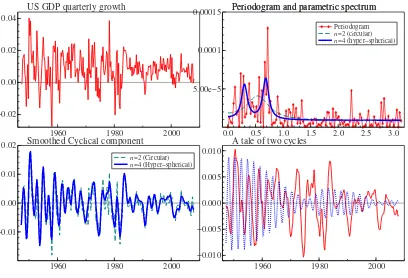
U.S., available for the sample period 1947:2-2008:4. The series is plotted in the top left hand panel of figure 1. We fit the cycle plus irregular model:yt=µ+ψt+ǫt,whereµis a constant,ǫt∼WN(0, σǫ2) andψtis the generalizedn-dimensional cyclical component given in (10)-(11).
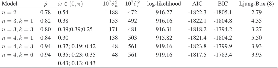
Table 1 presents the results of fitting cycle models of different dimension. The first (n= 2) is the cir-cular model described in (1); for the three-dimensional spherical model (n= 3) we consider the
specifi-cation withG(ω) =G12(ω)G13(ω)G23(ω), i.e. the same rotation angle defines the three Givens
matri-ces, and the specification with three different angles (k= 3), so thatG(ω) =G12(ω1)G13(ω2)G23(ω3).
Finally, we present the results for the four dimensional model with only one rotation angle (n= 4, k = 1), with six rotation angles, n = 4, k = 6, that is the model with transition matrix proportional to
G(ω) =G12(ω1)G13(ω2)G14(ω3)G23(ω4)G24(ω5)G34(ω6), along with a more parsimonious
speci-fication with onlyk= 3rotation angles, having
G(ω) =G12(ω1)G13(ω2)G14(ω1)G23(ω3)G24(ω2)G34(ω3).
Model ρˆ ωˆ ∈(0, π) 107
ˆ σ2
κ 10
7
ˆ σ2
ǫ log-likelihood AIC BIC Ljung-Box (8) n= 2 0.78 0.54 188 472 916.27 -1822.3 -1805.1 2.79
n= 3, k= 1 0.82 0.38 153 492 916.16 -1822.1 -1804.8 4.35
n= 3, k= 3 0.80 0.39;0.39;0.25 171 481 916.31 -1818.2 -1794.2 3.27
n= 4, k= 1 0.84 0.30 138 503 915.82 -1821.4 -1804.2 5.50
n= 4, k= 3 0.94 0.37; 0.19; 0.42 48 561 919.16 -1823.8 -1799.9 3.93
[image:13.595.75.539.107.222.2]n= 4, k= 6 0.94 0.35; 0.23; 0.35 48 561 919.16 -1817.5 -1783.4 3.93 0.43; 0.13; 0.43
Table 1: U.S. GDP quarterly growth. Estimation results
has the highest likelihood and the smallest AIC, and thus it would be selected according to this criterion. However, then= 2cycle is the best specification according to the BIC.
Figure 1 displays (top right panel) the sample spectrum and the parametric spectra implied by the
n = 2and n = 4, k = 3 models. The former peaks at a period of about 3 years. The second has two peaks at the spectral frequencies ζˆ1 = 0.30 and ζˆ2 = 0.69, corresponding to a five-year cycle
and to a short-run cycle with period of about two years. Although the smoothed estimates of the two cyclical components do not differ dramatically (then= 4resulting somewhat smoother), we think that
the interpretation of the bimodal spectrum is interesting. In the light of (12), the four dimensional cycle results from the sum of two cyclical components, the first, withζ1 close to 0.1π, describing a five-year
cycle, the second, with frequency corresponding to 2 years, describing a short-run cycle. The bottom right panel of figure 1, shows that the two-year plays a prominent role in the first part of the series, but then reduces prominently its amplitude. The five-year cycle plays a more important role at the end of the
sample.
The presence of a two-year cycle has been attested in the literature. For instance, the ARIMA(2,1,2)
estimated by Morley, Nelson and Zivot (2003) for the same series implies a cycle of 2.4 years.
5.2 Rainfall in Fortaleza
The series is the annual record of the number of centimeters of rainfall at Fortaleza, Brazil, for the period
1849-1992 (Source: Koopman et al., 2006). It provides an interesting case study for the detection and modelling of cycles in rainfall. Harvey and Souza (1987, HS) proposed the model
yt=µ+ψ1t+ψ2t+ǫt,
where ǫt ∼ WN(0, σǫ2) and ψit, i = 1,2, are two independent cycles specified as in (1). Maximum likelihood estimation (for the sample period up to 1979) gave two deterministic cycles with period 13 and 26 years; diagnostic checking and goodness of fit assessment led to conclude that the model provided
Figure 1: U.S. quarterly GDP growth rate. Original series, estimated cyclical component, decomposition into two cycles, sample and estimated spectrum.
1960 1980 2000
−0.02 0.00 0.02 0.04
US GDP quarterly growth
0.0 0.5 1.0 1.5 2.0 2.5 3.0 5.00e−5
0.0001
0.00015 Periodogram and parametric spectrumPeriodogram and parametric spectrum
Periodogram
n=2 (circular)
n=4 (hyper−spherical)
1960 1980 2000
−0.01 0.00 0.01
0.02 Smoothed Cyclical component
n=2 (Circular)
n=4 (Hyper−spherical)
1960 1980 2000
−0.010 −0.005 0.000 0.005 0.010
We are now going to fit the model
yt=µ+ψt+ǫt,
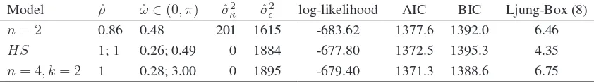
whereǫt ∼WN(0, σ2ǫ)andψtis the generalizedn-dimensional cyclical component given in (10)-(11), withn= 4, and compare the results with the HS specification and the circular cycle withn= 2. Model selection lead to the cyclical model withk= 2rotation angles and
G(ω) =G12(ω1)G13(ω1)G14(ω1)G23(ω2)G24(ω2)G34(ω2).
The estimation results, presented in table 2, confirm that also for the extended sample the HS specifi-cation with two deterministic cycles is preferable, although the BIC would point to the opposite
conclu-sion. The generalized four-dimensional cycle with two frequencies provides the best fit. The estimated
Model ρˆ ωˆ∈(0, π) σˆ2
κ ˆσ
2
ǫ log-likelihood AIC BIC Ljung-Box (8) n= 2 0.86 0.48 201 1615 -683.62 1377.6 1392.0 6.46
HS 1; 1 0.26; 0.49 0 1884 -677.80 1372.5 1395.3 4.35
[image:15.595.88.509.280.339.2]n= 4, k= 2 1 0.28; 3.00 0 1895 -679.40 1371.3 1388.6 6.75
Table 2: Rainfall in Fortaleza. Estimation results
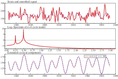
cycle and its spectral density (logarithms) is plotted are figure 2. The third panel compares the cycle with that arising from the HS model.
5.3 Mink-Muskrat Interaction
Our final illustration is an application of the elliptical cycle model to a famous bivariate time series, relating to the number of skins of minks and muskrats traded annually by the Hudson Bay Company in Canada from 1848 to 1909. The interest in this series lies in the fact that among the two species there
is a prey-predator relationship, which a sensible multiple time series model should capture. The series has been extensively investigated and discussed, by Bulmer (1974), Chan and Wallis (1978), Ter¨asvirta
(1985), Zhang, Yao, Tong and Stenseth (2003), among others.
As in Bulmer (1974) and Chan and Wallis (1978), the series are preliminarily transformed into log-arithms and detrended by removing a quadratic trend and linear trend respectively from the mink and
muskrat series. The detrended series are plotted in figure 3. Denoting the detrended muskrat and mink series respectively byy1t,andy2t, and lettingyt= [y1t, y2t]′, Chan and Wallis (CW) fitted the following vector ARMA(2,1) model with common AR polynomial:
ϕ(L)yt=Θ(L)ǫt, ǫt∼N(0,Σ),
whereǫt= [ǫ1t, ǫ2t]′.The maximum likelihood estimates of the parameters resulted:
ˆ
ϕ(L) = 1−1.28L+ 0.63L2,Θˆ(L) =
"
1−0.27L −0.79L 0.34L 1−0.75L
#
,Σˆ =
"
0.061 0.023 0.023 0.054
Figure 2: Annual rainfall series, Fortaleza (Brazil). Original series, estimated signal and cyclical com-ponent, and estimated log-spectrum for the modeln= 4, k= 2.
1860 1880 1900 1920 1940 1960 1980 2000
100 200
300 Series and smoothed signal
0.00 0.25 0.50 0.75 1.00 1.25 1.50 1.75 2.00 2.25 2.50 2.75 3.00
−5 0 5
10 Log−Spectrum of n=4 cycle model
1860 1880 1900 1920 1940 1960 1980 2000
125 150 175
Estimated cyclical components
The roots of the AR polynomial are complex and implying a damped oscillation with period 9.93 years.
As a measure of predictability, on an reverse scale, we can consider|Σˆ|, which equals 0.00275.
Since the above model could arise as the final equations form of a vector ARMA model (see Zellner
and Palm, 1974), CW proceed to fit the VAR(1) model
Φ(L)yt=ǫt, ǫt∼N(0,Σ),
which is the only VARMA model which can generate the above specification. The estimated coefficients
are
ˆ
Φ(L) =
"
1−0.79L 0.68L
−0.29L 1−0.51L
#
ˆ
Σ=
"
0.061 0.022 0.022 0.058
#
such that|Φˆ(L)|= 1−1.30L+0.60L2,which implies an AR(2) and conclude that the VAR(1)
specifica-tion provides a parsimonious and yet essential account of the interacspecifica-tions of the two series. In particular, the off-diagonal AR coefficients imply that an increase in the muskrat population (prey) is followed by an increase in the mink population (predator) a year later, and an increase in mink is followed by a decrease
in muskrat a year later. The estimated model implies that the two series display a cycle with a period of about 10 years, with the muskrat cycle leading the mink cycle by 2.4 years. With respect to the original
specification, the VAR(1) model yields an higher value of the (un)predictability,|Σˆ|, which now equals 0.00305, but has fewer parameters.
In the place of an unrestricted VAR(1) model we fit and compare two bivariate cycle models, the
spherical cycle model (SCM) and the elliptical (ECM), which can be regarded as two constrained version of the final model fitted by CW. The SCM is specified as follows:
yt=ρG12(ω)yt−1+ǫt, ǫt∼N(0,Σ),
whereas the ECM is
yt=E(ω)yt−1+ǫt, ǫt∼N(0,Σ),
where was given in 5, i.e.
E(ω) =
"
αcosω αsinω
−βsinω βcosω
#
.
Therefore, the ECM encompasses the SCM, which arises whenα=β(=ρ).
Table 3 displays some estimation results. The estimated values of α and β resulted respectively
1.00 and 0.60, whereas the cycle frequency is estimated equal to 0.63. The hypothesisH0 : α = β is
strongly rejected. The results provide strong support for the elliptical cycle specification. The second panel of figure 3 suggest that this is the case since the variability of muskrat population is larger than that
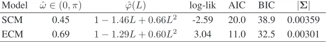
Model ωˆ ∈(0, π) ϕˆ(L) log-lik AIC BIC |Σ| SCM 0.45 1−1.46L+ 0.66L2
-2.59 20.0 38.9 0.00359 ECM 0.69 1−1.29L+ 0.60L2
[image:18.595.139.465.108.150.2]3.04 11.0 32.5 0.00301
Table 3: Mink-Muskrat bivariate time series. Estimation results
The estimated autoregressive matrix polynomial and prediction error covariance matrix for the ECM are very similar to the unrestricted VAR(1) model fitted by CW:
I−E(ω)L=
"
1−0.81L 0.59L
−0.36L 1−0.49L
#
,Σˆ =
"
0.061 0.021 0.021 0.056
#
.
The implied final equations form hasϕˆ(L) = |I2 −Eˆ(ω)L|almost identical to that implied by CW’s
VAR(1) model (see table 3), and the predictability measure is about the same (actually, it is slightly
smaller). Moreover, it has a parameter less and thus ECM would be preferred to the VAR(1) by an information criterion.
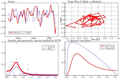
The bottom right hand panel of figure 3 displays the two parametric spectra implied for the two series
by the ECM specification, which have the following expressions. Denoting byσij the generic element ofΣ,
f11(λ) = 1 2π
σ11(1−2βcosωcosλ+β2cos2ω) +σ12(2αsinωcosλ−αβsin 2ω) +σ22(α2sin2ω) 1 +α2β2+ (α+β)2cos2ω−2(α+β)(1 +αβ) cosωcosλ+ 2αβcos(2λ) ,
f22(λ) = 1 2π
σ11(β2sin2ω) +σ12(αβsin 2ω−2βsinωcosλ) +σ22(1−2αcosωcosλ+α2cos2ω) 1 +α2β2+ (α+β)2cos2ω−2(α+β)(1 +αβ) cosωcosλ+ 2αβcos(2λ) .
The spectral peak is located at a frequency corresponding to a ten year cycle.
The last panel shows the spectral coherence and the phase between the two series, computed respec-tively asℜ{f12(λ)}2+ℑ{f12(λ)}2andarctan{−ℑ{f12(λ)}/ℜ{f12(λ)}}whereℜandℑare the real
and imaginary parts of the cross-spectrum:
f12(λ) = 1 2π
σ11s11+σ12s12+σ22s22
1 +α2β2+ (α+β)2cos2ω−2(α+β)(1 +αβ) cosωcosλ+ 2αβcos(2λ),
where s11 = −βsinωeıλ +β2sinωcosω, s12 = 1− cosω(αeıλ +βe−ıλ) +αβcos 2ω, s22 =
αsinωe−ıλ−α2sinωcosω.
6
Conclusions
The paper has proposed multivariate and elliptical extensions of the traditional circular cycle model. The empirical applications have pointed out under what circumstances these extensions can be fruitful. Other
Figure 3: Mink-Muskrat bivariate time series. Original series, phase plot, univariate spectra, coherence and phase diagram implied by the elliptical cycle model.
1860 1880 1900
−1.5 −1.0 −0.5 0.0 0.5
1.0 Series
Muskrat Mink
−1.6 −1.2 −0.8 −0.4 0.0 0.4 0.8 1.2 1.6
−1.6 −1.2 −0.8 −0.4 0 0.4 0.8 1.2 1.6 Muskrat
Mink
Time Plot of Mink vs Muskrat
0.0 0.5 1.0 1.5 2.0 2.5 3.0 0.1
0.2
0.3 Sample and parametric spectra implied by ECM
Muskrat Mink
0.0 0.5 1.0 1.5 2.0 2.5 3.0 0.5
1.0
Coherence and phase
There are some open issues that this paper has left unresolved and that we leave for future research.
Appendix
A
Proof of Proposition 1
We aim at locating the value ofλfor which the power spectrum of the circular stochastic cycle (1),
f(λ) = σ 2
k
2π
1 +ρ2−2ρcosωcosλ
1 +ρ4+ 4ρ2cos2ω−4ρ(1 +ρ2) cosωcosλ+ 2ρ2cos(2λ),
is maximum. First notice that
lim
ρ→0f(λ) =
σ2
k
2π and ρlim→1f(ω) =∞,
since the (squared) denominator of the above equation is null for
cosλ= (1 +ρ
2) cosω∓sinωp
−(1−ρ2)2
2ρ ,
i.e. forρ= 1andλ=ω.Whenρ∈(0,1), the first order conditions give:
2ρcosωsinλ(1 +ρ4+ 4ρ2cos2ω−4ρ(1 +ρ2) cosωcosλ+ 2ρ2cos(2λ))+
− (4ρ(1 +ρ2) cosωsinλ−4ρ2sin(2λ))(1 +ρ2−2ρcosωcosλ) = 0.
Equivalently
sinλ£
2ρcosω(1 +ρ4+ 4ρ2cos2ω)−(2ρcosω)4ρ(1 +ρ2) cosωcosλ+
+ (2ρcosω2ρ2cos(2λ))−(4ρ(1 +ρ2) cosω−4ρ22 cos(λ))(1 +ρ2−2ρcosωcosλ)¤
= 0,
which is null for λ = 0(this is a relative minimum). Let us consider the other solutions. By some algebra, the above equation can be written as the second order equation incosλ,
4ρ2cosωcos2λ−2ρ(1 +ρ2)2 cosλ−cosω(1 +ρ4+ 4ρ2cos2ω) + 2ρ2cosω+ 2(1 +ρ2)2cosω= 0.
Noticing that−1−ρ4−6ρ2 =−(1 +ρ2)2−4ρ2and using some algebra and trigonometric identities,
one can obtain the roots of the above equations as
cosλ1,2 =
(1 +ρ2)∓sinωp
(1 +ρ2)2−4ρ2cos2ω 2ρcosω
The quantity under square root is always positive forρ <1and there is only one admissible solution, in modulus smaller than one, that can be expressed as
cosλmax=
1 +ρ2 2ρcosω
Ã
1−sinω
s
1− 4ρ 2
(1 +ρ2)2 cos2ω !
.
The overall conclusion is that, for ρ that tends to unity, the spectrum reaches its maximum at a
B
Proof of Proposition 2
The proof is analogue to the proof of proposition 1, provided thatαandβ are considered in place ofρ, so we just summarise the main steps. Differentiating (6) with respect toλand equating to zero gives
sinλ(8αβ2cosωcos2λ−2Acosλ−B) = 0,
whereA= 4αβ(1 +R2),B= 2βcosω(1 +α2β2+ (α+β)2cos2ω−2β)−2(α+β)(1 +αβ)(1 + R2) cosω) andR2 = α2sin2ω+β2cos2ω, from which the relative minimum inλ= 0. Solving the
second order equation incosλgives
cosλmax= 1 +R
2
2βcosω
³
1∓p1 +Ccos4ω−Dcos2ω´,
whereC = βα(1+(α+Rβ2)2
)2,D=−
µβ
α+αβ 3−
2β2
(1+R2
)2 −
1+αβ+βα+β2
1+R2
¶
,C, D >0. Of the two solutions, only the
one with the minus gives a value for the cosine which is smaller than one. Using trigonometric identities
and collecting terms, we rewrite the above equation to have the solution given in proposition 4.
C
Proof of Proposition 3
To obtain the reduced form ofψtin (8), we start by writing
ψt=Z′ρGz(ξ)Zψt−1+κt
which, after some algebra, is equivalent to
˜
ψt= (I−ρGz(ξ)L)
∗
det(I−ρGz(ξ)L)
κt,
whereψ˜t=Zψtand the superscript∗denotes the adjoint, or adjugate, of a matrix. The above expression allows us to conveniently derive the reduced form of the reparameterized processψ˜t. In fact, for all the components ofψ˜t, i.e. the processesψ˜t,ψ˜t†andψ˜
‡
t, the autoregressive polynomial is det(I−ρGz(ξ)L) =
(1−ρL)(1−2ρcosξL +ρ2L2), whereas the moving average polynomial is the j-th row of (I −
ρGz(ξ)L)∗, forj= 1,2,3. The adjoint is here obtained as
(I−ρGz(ξ)L)∗=p1I+p2(I−ρGz(ξ)L) +p3(I−ρGz(ξ)L)2
where thepjare the coefficients ofxjin the characteristic polynomialp(x) =|(I−ρGz(ξ)L)−xI|, i.e.
p1 = 3 +ρ2L2+ 2ρ2cosξL2−4ρcosξL−2ρL
p2 = 2ρcosξL+ρL−3
which follows by the Cayley-Hamilton theorem(p(I−ρGz(ξ)L) =0)and by the fact thatp0=−|I−
ρGz(ξ)L|(Lancaster and Tismenetsky, p. 157, Theorem 2, and p. 165, Ex. 8). With some algebra,
(I−ρGz(ξ)L)∗ =I+ £
(1 + 2 cosξ)(I−Gz(ξ)) +Gz(ξ)2 ¤
ρ2L2−[(1 + 2 cosξ)I−Gz(ξ)]ρL
whose first row timesκtis equal to
e′1(I−ρGz(ξ)L)∗κt = {1−(1 + cosξ)ρL+ [(1 + 2 cosξ)(1−cosξ) + cos(2ξ)]ρ2L2}κt+
+{ρsinξL+ [−(1 + 2 cosξ) sinξ+ sin(2ξ)]ρ2L2}κ†
t,
wheree1= [1 0 0]′.Hence, the reduced form ofψ˜tis
(1−ρL)(1−2ρcosξL+ρ2L2) ˜ψt={1−(1 + cosξ)ρL+ cosξρ2L2}κt+{ρsinξL−sinξρ2L2}κ†t.
Collecting terms we find
(1−ρL)(1−2ρcosξL+ρ2L2) ˜ψt= (1−ρL)(1−cosξρL)κt+ (1−ρL)(ρsinξL)κ†t,
i.e.,ψ˜tis observationally equivalent to the first order stochastic cycle (1).
The reduced form of the auxiliary processesψ˜†tandψ˜‡tare derived in an analog way and are given by the ARMA(2,1) process(1−2ρcosξL+ρ2L2) ˜ψ†
t =−(ρsinξL)κt+ (1−cosξρL)κ†t and the AR(1) process(1−ρL) ˜ψt‡=κ‡t, respectively.
Finally,ψt=e′1Z′ψ˜tis the ARMA(3,2) process given in (9). The spectrum is obtained by the Fourier transform of the spectral generating function for an ARMA process, see Harvey (1989, pag. 59). This concludes the proof of proposition 2.
D
Proof of Proposition 4
Let us write (10) as
ψt= (I−ρG(ω)L)
∗
det(I−ρG(ω)L)κt.
Ifnis even, then det(I−ρG(ω)L) = Q
n 2
h=1(1−2ρcosζhL+ρ2L2)which follows by the fact that
the spectrum ofG(ω)is the set{eıζ1, eıζ2, . . . , eıζn}, whereζ
2h = −ζ2h−1,forh = 1,2, . . . ,n2,and
tr(G(ω)) = 2Pn2
h=1cosζh. The adjoint is
(I−ρG(ω)L)∗=− n X
j=1
(−1)n−jsn−j(I−ρG(ω)L)j−1,
where we have used the Cayley-Hamilton theorem, as in the proof of proposition 3, withpj = (−1)n−jsn−j andsn−j being the symmetric function of the eigenvalues ofI−ρG(ω)L, defined to be the sum of the product of the eigenvalues takenn−jat a time, i.e.
sn−j =
X
1≤i1<i2<...<in−j≤n
(Meyer, 2000, p. 494). Writing(I−ρG(ω)L)j−1 =V(I−ρΞL)j−1VH, whereΞ= diag (eıζ1, eıζ2, . . . , eıζn),
and taking the first row, we obtain (12).
Ifnis odd, then the spectrum ofG(ω)is the set{eıζ1, eıζ2, . . . , eıζn−1,1}, whereζ
2h =−ζ2h−1,for
h= 1,2, . . . ,n−21with tr(G(ω)) = 1+2Pn−
1 2
h=1cosζh, the adjoint is(I−ρG(ω)L)∗= Pn
j=1(−1)n−jsn−j(I−
ρG(ω)L)j−1and, consequently,
(1−ρL)
n−1 2
Y
h=1
(1−2ρcosζhL+ρ2L2)ψt,1=
n X
j=1
n X
i=1
n X
k=1
(−1)n−jsn−jv1i(1−ρeıζiL)j−1vkiκt,k,
References
Bulmer M.G. (1974), A statistical analysis of the 10-year cycle in Canada, Journal of Animal Ecol-ogy, 43, 701718.
Chan W.-Y. T. and Wallis K.F. (1978), Multiple Time Series Modelling: Another Look at the Mink-Muskrat Interaction, Applied Statistics, 27, 2, 168-175.
Doornik, J.A. (2006),Ox. An Object-Oriented Matrix Programming Language, Timberlake Consul-tants Press, London.
Durbin, J., Koopman S.J. (2001), Time Series Analysis by State Space Methods, Oxford University Press.
Givens W. (1958), Computation of plane unitary rotations transforming a general matrix to triangular form,SIAM Journal, 6, 1, 2650.
Goldstein H. (1980),Classical Mechanics, second edition, Addison-Wesley.
Golub G.H. and van Loan C.F. (1996),Matrix Computations, third edition, The John Hopkins Uni-versity Press.
Gray, S., Zhang, N.-F., Woodward, W.A., 1989. On generalized fractional processes. Journal of Time Series Analysis, 10, 233-257.
Hannan E.J. (1964), The Estimation of a Changing Sesasonal Pattern,Journal of the American Sta-tistical Association, 59, 308, 1063-1077.
Harvey A.C. (1985), Trends and Cycles in Macroeconomic Time Series, Journal of Business and Economics Statistics, 3, 3, 216-227.
Harvey A.C. (1989), Forecasting, Structural Time Series Models and the Kalman Filter, Cambridge University Press.
Harvey A.C. and Jaeger A. (1993), Detrending, Stylized Facts and the Business Cycle, Journal of Applied Econometrics, 8, 231-247.
Harvey A.C. and Souza R.C. (1987), Assessing and Modeling the Cyclical Behavior of Rainfall in
Northeast Brazil,Journal of Climate and Applied Meteorology, 26, 10, 1339-1344.
Harvey A.C. and Trimbur, T.M. (2003), General Model-based Filters for Extracting Cycles and Trends
Haywood J. and Tunnicliffe Wilson, G. (2000), An Improved State Space Representation for Cyclical
Time Series,Biometrika, 87, 3, 724-726.
Kendall M.G. (1945), On the Analysis of Oscillatory Time-Series, Journal of the Royal Statistical Society, Series B, 108, 1/2, 93-141.
Koopman S.J., Harvey, A.C., Doornik, J.A. and Shephard, N. (2006), STAMP: Structural Time Series Analyser, Modeller and Predictor, Timberlake Consultants Press.
Lancaster P. and Tismenetsky M. (1985),The Theory of Matrices, Academic Press. L¨utkepohl H. (2006),New Introduction to Multiple Time Series Analysis, Springer. Meyer C.D. (2000),Matrix Analysis and Applied Linear Algebra, SIAM.
Morgan M.S. (1990),The History of Econometric Ideas. Cambridge University Press, Cambridge, U.K.
Morley J.C., Nelson C.R., Zivot E. (2003), Why Are the Beveridge-Nelson and Unobserved Com-ponents Decompositions of GDP So Different?,The Review of Economics and Statistics, 85, 2, 235-243.
Ter¨asvirta, T. (1985), Mink and Muskrat interaction: a structural approach, Journal of Time Series Analysis, 6, 3, 171-180.
Tong H., Lim K.S. (1980), Threshold Autoregression, Limit Cycles and Cyclical Data,Journal of the Royal Statistical Society, Series B, 42, 3, 249-292.
Trimbur, T.M. (2005), Properties of Higher Order Stochastic Cycles,Journal of Time Series Analysis, 27, 1, 1-17.
West, M., Harrison, J. (1989), Bayesian Forecasting and Dynamic Models, 1st edition, New York, Springer-Verlag.
West, M., Harrison, J. (1997),Bayesian Forecasting and Dynamic Models, 2nd edition, New York, Springer-Verlag.
Yule, G.U. (1927), On a Method of Investigating Periodicities in Disturbed Series, with Special Ref-erence to Wolfer’s Sunspot Numbers,Philosophical Transactions of the Royal Society of London. Series A, Containing Papers of a Mathematical or Physical Character, 226, 1, 267-298.
Zellner A., Palm F. (1974), Time series analysis and simultaneous equation econometric models,
Zhang W., Yao Q., Tong H.,Stenseth N.C. (2003), Smoothing for Spatiotemporal Models and Its