Munich Personal RePEc Archive
Relevant States and Memory in Markov
Chain Bootstrapping and Simulation
Cerqueti, Roy and Falbo, Paolo and Pelizzari, Cristian
University of Macerata, Italy, University of Brescia, Italy, University
of Brescia, Italy
March 2010
Online at
https://mpra.ub.uni-muenchen.de/46254/
Relevant States and Memory in Markov Chain Bootstrapping
and Simulation
Roy Cerqueti
Universit`a degli Studi di Macerata - Dipartimento di Istituzioni Economiche e Finanziarie
Via Crescimbeni, 20 - 62100 Macerata MC - Italy. E-mail: [email protected]
Paolo Falbo
Universit`a degli Studi di Brescia - Dipartimento Metodi Quantitativi
Contrada Santa Chiara, 50 - 25122 Brescia BS - Italy. E-mail: [email protected].
Cristian Pelizzari
Universit`a degli Studi di Brescia - Dipartimento Metodi Quantitativi
Contrada Santa Chiara, 50 - 25122 Brescia BS - Italy
Corresponding author. Tel.: +39 030 2988516. Fax: +39 030 2400925. E-mail: [email protected].
Abstract
Markov chain theory is proving to be a powerful approach to bootstrap highly nonlinear
time series. In this work we provide a method to estimate the memory of a Markov chain (i.e.
its order) and to identify its relevant states. In particular the choice of memory lags and the
aggregation of irrelevant states are obtained by looking for regularities in the transition
prob-abilities. Our approach is based on an optimization model. More specifically we consider two
competing objectives that a researcher will in general pursue when dealing with bootstrapping:
preserving the “structural” similarity between the original and the simulated series and assuring
a controlled diversification of the latter. A discussion based on information theory is developed
to define the desirable properties for such optimal criteria. Two numerical tests are developed
to verify the effectiveness of the method proposed here.
MSC classification: 60J10, 60J20, 60J22, 62B10, 62F40, 91G60.
1
Introduction
In the financial literature, starting from the tests on efficient market hypothesis and the technical
analysis (e.g., Brock et al., 1992; Sullivan et al., 1999), bootstrap procedures have been applied
intensively to solve a wide variety of problems. Following such a spread interest, several
method-ological contributions have appeared to improve the initial bootstrap method advanced by Efron
(1979), even if the basic idea remains unchanged (e.g., see the methodological discussion on the
classical bootstrap methods in Freedman, 1984; Freedman and Peters, 1984; Efron and Tibshirani,
1986, 1993). In particular, the heart of the bootstrap consists of resampling some given observations
with the purpose of obtaining a good estimation of statistical properties of the original population.
However, an important restriction to the classical bootstrap methods is that the original population
must be composed of independent identically distributed observations. In the case of time series
taken from the real life, this condition is hardly true. When such hypothesis is not true, a theoretical
model for the data is required and the bootstrap is then applied to the model errors.
A new group of bootstrapping methods has been advanced to reduce the risk of mis-specifying the
model. To this group belong the so calledblock,sieve, and thelocal methods of bootstrapping (see
B¨uhlmann, 2002, for a comparison of these methods). The methods are nonparametric, and assume
that observations can be (time) dependent.
This category of literature has increased in a relatively recent period of a new method of
bootstrap-ping based on Markov chain theory. The major advantage of this approach is that it is entirely
data driven, so that it can smoothly capture the dependence structure of a time series, releasing a
researcher from the risk of wrongly specifying the model, and from the difficulties of estimating its
parameters.
The limitation connected to Markov chains is of course that they are naturally unsuitable to model
discrete-valued processes. This is an unfortunate situation, since several phenomena in many areas
of research are often modeled through continuous-valued processes. In the economic and financial
literature, there are plenty of cases of continuous-valued processes showing complex behaviors, where
observations appear to depend nonlinearly from previous values. It is well known that in the
finan-cial markets, next to technological and organizational factors, psychology and emotional contagion
introduce complex dynamics in driving the expectations on prices (e.g., think to the terms popular
in the technical analysis such as “psychological thresholds”, “price supports”, “price resistances”,
etc.). In such cases, guessing the correct model for complex continuous-valued stochastic processes
is highly risky.
To overcome this risk, a researcher in the need of bootstrapping or simulating a continuous-valued
stochastic process could in principle resort to partitioning its support, obtaining a discretized version
of it, and then apply Markov chain bootstrapping or simulation techniques to model brilliantly any
how to organize anefficient partition of the process support. Indeed in the absence of some guide,
fixing arbitrarily a partition excessively refined or raw involves different kinds of drawbacks, ranging
from insufficient diversification of the simulated trajectories to unsatisfactory replication of the key
features of the stochastic process.
In this paper we develop an original general approach to determine the relevant states and the
mem-ory (i.e. the order) of a Markov chain, keeping in mind the major problems connected to applying
Markov chain bootstrapping and simulation to continuous-valued processes.
There is a wide literature which has dealt with the analysis of states and memory of a Markov chain
for resampling purposes, which we review in the following section. It is quite important to notice
that such literature has mainly focused on the estimation of the order of a Markov chain more than
it has done to discriminate the relevant states, and this is due to the fact that Markov chains are
discrete-valued processes, where the states are usually taken as equally important.
From our perspective, focusing on the relevant states is crucial if we want to consider the discretized
versions of complex continuous-valued processes. As mentioned previously, it is frequent in economic
and financial markets that some observed states, or combinations of them, are more relevant than
others in determining the future evolution of the process. In other words, not all the partitions of
the support of a continuous-valued process are suitable to capture the relevant information about its
dependence structure. Finding the optimal ones is therefore crucial to apply correctly the
method-ology of Markov chain bootstrapping and simulation. However bootstrapping requires to take care
of an aspect, which we deal with here explicitly and which is not as critical with simulation. In
Markov chain bootstrapping the probability to re-generate large portions of the original series is a
serious drawback, especially when the number of states and order of the Markov chain increase and
transition probabilities get close to unity (the limiting case is the repetition of the entire original
series). We deal with this diversification problem in our model.
The approach we propose in this paper is based on the joint estimation of the relevant states and
of the order of a Markov chain and consists of an optimization problem. The solution identifies the
partition which groups the states with the most similar transition probabilities. In this way the
resulting groups emerge as the relevant states, that is the states which significantly influence the
conditional distribution properties of the process. Furthermore, as we will show, our approach is
information efficient in the sense of Kolmogorov (1965), that is it searches for the partition which
minimizes the information loss. Our optimization problem includes also the “multiplicity” constraint
which controls for a sufficient diversification of the resampled trajectories.
Our work contributes to the literature on Markov chain bootstrapping in various ways.
Firstly, we develop a method to estimate the parameters of a Markov chain dedicated to bootstrap
via constrained optimization. When the threshold defining the multiplicity constraint is let to vary,
solu-tions.
Secondly, we propose a non hierarchical approach, which means that a non sequential search of the
order of the Markov chain is performed. More precisely, if some states are grouped at a given time lag
w, then they are not forced to stay together at farther time lagsw+r(withr >0). This “freedom”
adds flexibility in modeling the dependence structure of a Markov chain and, to our knowledge, our
approach is the first in the literature on Markov chain bootstrapping and simulation to abandon
hierarchical grouping. Such a feature is not of secondary importance, since it allows to model a
Markov chain with non monotonically decreasing memory.
Thirdly, comparing to the bootstrap literature developed in econometrics and applied statistics, our
proposal treats states as if they were of qualitative nature, and the search of efficient partitions is
based only on transition probabilities. In other words, no distance between the values of the different
states is used in the decision of merging them. Again, this approach allows a higher flexibility in the
identification of the relevant states and an increased capacity to capture the dynamics of a Markov
chain.
Fourthly, this paper provides the theoretical grounds for Markov chain bootstrapping and simulation
of continuous-valued processes. To the best of our knowledge, this is the first attempt to extend
Markov chain bootstrapping and simulation in this sense. Our search for the relevant states supplies
the levels where the process modifies significantly its dynamics (i.e. its expected value, its variance,
etc.). Hence, it is designed to minimize the information loss deriving from aggregating the states,
so it helps maintaining highly complex nonlinearities of the original process.
Fifthly, we introduce two new non entropic measures of the disorder of a Markov chain process, and
we study their main properties.
The paper is organized as follows. Section 2 reviews the relevant literature on Markov chain
boot-strapping. Section 3 introduces the settings of the problem. Section 4 discusses some theoretical
properties of the criteria used here to select the optimal dimension of a Markov chain transition
probability matrix. Section 5 discusses some methodological issues. In Section 6 the criteria are
applied to two examples. Section 7 concludes.
2
A Bibliography Review on Markov Chain Bootstrapping
It is possible to group different contributions on resampling procedures based on Markov chain
the-ory.
A first major category is concerned with processes that are not necessarily Markov chains. A series
of stationary data is divided into blocks of length l of consecutive observations; bootstrap samples
are then generated joining randomly some blocks. The seminal idea appears first in Hall (1985)
starting with K¨unsch (1989) and Liu and Singh (1992). In Hall et al. (1995), B¨uhlmann and K¨unsch
(1999), Politis and White (2004), and Lahiri et al. (2007), the selection of the parameterl -a crucial
point of this method- is driven by the observed data.
Many variants of the block bootstrap method exist by now; standard references include Politis and
Romano (1992) for theblocks-of-blocks bootstrap, Politis and Romano (1994) for thestationary
boot-strap, and Paparoditis and Politis (2001a, 2002a) for thetapered block bootstrap. For a survey, see
Lahiri (2003). Despite the block based bootstrap methods have been developed to get over the
problem of dependence disruption, they only partially succeed in their goal. Indeed they pass from
the loss of dependency among data to that among blocks.
A second category relies to Markov chains (or processes) with finite states and faces explicitly the
problem of maintaining the original data dependency. Earlier approaches to bootstrap Markov
chains were advanced by Kulperger and Prakasa Rao (1989), Basawa et al. (1990), and Athreya and
Fuh (1992), and have been further investigated in Datta and McCormick (1992). This second group
is more closely related to our work, since it focuses on the transition probabilities of a stationary
Markov chain (or process), as we also do here. It is useful to distinguish some different approaches.
Thesieve (Markov) bootstrapmethod was first advanced by B¨uhlmann (1997); it consists of fitting
Markovian models (such as an AR) to a data series and resampling randomly from the residuals.
This idea has been further developed in B¨uhlmann (2002), where the variable length Markov chain
sieve bootstrap method is advanced. This is an intriguing approach since in nature it happens that
only “some” sequences of states (i.e. paths) tend to reappear in an observed sequence more than
others and to condition significantly the process evolution. However this method proceeds in a
hier-archical way to search for the relevant paths, which can be a severe limitation when time dependence
is not monotonically decreasing.
Still in the framework of Markov processes, Rajarshi (1990) and Horowitz (2003) estimate the
tran-sition density function of a Markov process using kernel probability estimates. The idea of using
kernels is adopted also by Paparoditis and Politis (2001b, 2002b), which advance the so calledlocal
bootstrap method. This method rests on the assumption that similar trajectories will tend to show
similar transition probabilities in the future. However it is not uncommon to observe empirical
contradiction to such hypothesis. Besides, the number of time lags to be observed to compare
tra-jectories has to be chosen arbitrarily.
Anatolyev and Vasnev (2002) propose a method (Markov chain bootstrap) based on a finite state
discrete Markov chain. Similarly to what we do here, the authors partition the state space of the
series intoI sets (bins). While some interesting estimation properties of the bootstrap method are
shown, the bins are formed simply distributing the ordered values evenly in each of them. Besides,
an arbitrary number of time lags is also fixed to bound the relevant path length.
Athreya and Fuh (1992) and Datta and McCormick (1993), and has been further analyzed by Bertail
and Cl´emen¸con (2006, 2007). This method focuses on a chosen recurring state (atom) and the
con-secutive observations between departure from and return to the atom (cycle or block). Bootstrapping
is then accomplished by sampling at random from the observed cycles. This method reconciles the
gap between Markov chain bootstrapping procedures and block bootstrapping, with the important
difference that the cutting points (used to form the blocks) in the Markov chain approach are not
chosen at random, but are data driven. Besides, it does not need to explicitly estimate the transition
probabilities of the observed process. However this relies heavily on the identification of the atom,
which is unfortunately unknown.
The problem of estimating the relevant states and the order of a Markov chain process for
boot-strapping purposes can also be related to the information theory literature, with particular reference
to the data compression analysis. In general terms, data compression problems rely on flows of data
generated by a process with a finite alphabet, like a finite state Markov chain. The criteria adopted
for estimating the relevant parameters of a finite state process include, for example, the AIC (Akaike
Information Criterion, Akaike, 1970), the BIC (Bayesian Information Criterion, Schwarz, 1978), and
the MDL principle (Minimum Description Length principle, Rissanen, 1978). Each criterion consists
of two parts: an entropy-based functional and a penalty term depending on the number of
parame-ters, both to be minimized.
The link between bootstrapping and data compression analysis can be stated as follows. As already
stressed above, a key point in bootstrap problems consists in generating simulated series keeping
the relevant statistical properties of the original one and avoiding the risk of exactly replicating the
original series. Under the data compression theory point of view, the former aspect can be
trans-lated into the minimization of the entropy-type distance, while the latter is formalized through the
minimization of the penalty term.
In this respect, we estimate the relevant parameters of a Markov chain process for bootstrapping
purposes via a constrained optimization problem. Rather than entropy, two specific distances based
on the transition probabilities are introduced and minimized. The introduction of non entropic
measures is based on three reasons: first of all, there is no consensus on a preferable entropy
mea-sure among the several available (Ullah, 1996; Cha, 2007); secondly, as we will see, our distance
indicators are close to usual dispersion measures, analytically simple, and we could prove easily for
them the minimal properties required to disorder measures discussed in Kolmogorov (1965); lastly,
the introduction of two new measures is an extension of the literature on information theory. A
constraint is also introduced which corresponds to minimizing the penalty term.
Starting from Rissanen (1978), Rissanen (1983), Rissanen and Langdon Jr. (1981), and Barron et al.
(1998), which first showed the strict link between coding and estimation, literature on data
Of particular interest for us are Rissanen (1986), Ziv and Merhav (1992), Weinberger et al. (1992),
Feder et al. (1992), Liu and Narayan (1994), and Weinberger et al. (1995). These works study the
class of finite-state sources and, among other results, develop methods for estimating their states;
an important example of a finite-state source is a Markov chain with variable memory, also called
variable length Markov chain (VLMC) (see B¨uhlmann and Wyner, 1999; B¨uhlmann, 2002). As its
name suggests, aVLMC is characterized by a variable order depending on which state verifies at
past time lags. Starting from time lag 1, states are differentiated only if they contribute to
dif-ferentiate future evolution, otherwise they are lumped together. Farther time lags are considered
only for those states showing additional prediction power. In the end, such approach identifies a
Markov model whose memory changes depending on the trajectory followed by the process. This
approach proves to be computationally efficient, as it allows a strong synthesis of the state space.
As a further application, the method can be used to develop a bootstrap engine (VLMC bootstrap),
which is more user-friendly and attractive than the block bootstrap (K¨unsch, 1989). B¨uhlmann and
Wyner (1999) and B¨uhlmann (2002) are strongly related to our work, as the reduction to a minimal
state space is also an objective of the present study. The main difference in our proposal consists
of a non hierarchical selection of the relevant time lags, in the sense that we do not condition the
relevance of farther time lags to depend on that of the closer ones.
Merhav et al. (1989), Finesso (1992), Kieffer (1993), Liu and Narayan (1994), Csisz´ar and Shields
(2000), Csisz´ar (2002), Morvai and Weiss (2005), Peres and Shields (2008), and Chambaz et al.
(2009) consider the problem of the estimation of the order of a Markov chain, assuming that the
states are all relevant at all the time lags up to the estimated order. However, in some applications
a satisfactory estimation of the relevant states is even more important than a precise estimation of
the “memory” of the process. We refer, for example, to the bootstrapping of series with regimes
characterizing the dynamics of different processes in economics and finance.
3
The model
Let us consider an evolutive observable phenomenon, either continuous or discrete. We suppose that
we observeNrealizations homogeneously spaced in time and we introduce the set of the time-ordered
observations of the phenomenon,E={y1, . . . , yN}. They1, . . . , yN are understood as the values of a discrete process or as the labels of a discretized continuous process. There existJN ≥1 distinct statesa1, . . . , aJN ∈E. The corresponding subsets of E, denoted asE1, . . . , EJN, and defined as:
Ez={yi ∈E|yi=az}, z= 1, . . . , JN,i= 1, ..., N
constitute a partition of E. Moreover, fixed z = 1, . . . , JN, then the frequency of state az in the
We now consider a time-homogeneous Markov chain of orderk≥1, denoted as{X(t), t≥0}, with state spaceA. To ease the notation, in the following we will simply write Markov chain instead of
time-homogeneous Markov chain. Thek-lag memory of the Markov chain implies that the transition
probability matrix should account for conditioning to trajectories of length k. Therefore, we refer
hereafter to ak-path transition probability matrix.
We deal in our paper with a couple of questions related to finding the Markov chain which best
describes the observed seriesE:
• Which is the optimalk?
• Which is the optimal clustering ofA for each time lagw, with w= 1, ..., k?
It is important to notice that, though the second question focuses primarily on the search of the
relevant states, it actually also addresses the analysis of the memory of a Markov chain. Indeed if the
optimal clustering at time lagwreturns many or just a few classes, we obtain an information about
the relevance of that time lag. Few or no classes will in general signal low or no conditioning power.
On the contrary the presence of many classes will signal higher relevance. Since the clustering is
operated independently for each time lag, this approach can return a distribution of the relevance
of the memory of a Markov chain over all the time lags, which need not to be in decreasing order
from 1 to k. We introduce a measure of relevance, or “activity”, for a time lag later in Section 5
(Methodological issues).
Let us consider az ∈ A andah = (ah,k, ..., ah,1)∈ Ak. The row vector ah is the ordered set of k statesah,w∈A,w= 1, ..., k, listed, in a natural way, from the furthest to the closest realization of the chain. This ordering of the realizations will be maintained throughout the paper. The Markov
chain has stationary probabilities:
P(ah) =P(X(t) =ah,1, . . . , X(t−k+ 1) =ah,k), (1)
and transition probability fromah to stateaz:
P(az|ah) =P(X(t) =az|X(t−1) =ah,1, . . . , X(t−k) =ah,k). (2)
According to Ching et al. (2008), we estimate the transition probability P(az|ah) by using the empirical frequencies f(az|ah) related to the phenomenon. For the sake of simplicity, we avoid introducing throughout the paper a specific notation for the estimates of the probabilities, therefore
we estimateP(az|ah) by
P(az|ah) =
f(az|ah)
∑
j:aj∈Af(aj|ah), if ∑
j:aj∈Af(aj|ah)̸= 0
0, otherwise
Analogously,P(ah) is estimated by
P(ah) =
∑
j:aj∈Af(aj|ah) ∑
b:ab∈Ak ∑
j:aj∈Af(aj|ab)
.
Thek-path transition probability matrix of{X(t), t≥0}, which is defined by the quantities in (2), is estimated by the quantities in (3).
Let us now introduce the set Λ of the partitions of A. A generic element λ ∈ Λ can be written as λ={A1, . . . , A|λ|}, where|λ| is the cardinality of λ, with 1≤ |λ| ≤JN, and{Aq}q=1,...,|λ| is a partition of nonempty subsets ofA. The cardinality of Λ isB(JN), i.e. the Bell number1 of theJN
elements in setA.
Extending our notation to a multidimensional context, we consider the set Λk of k-dimensional partitions. The setΛkcontains the partitions we will focus on in the present paper. Ak-dimensional partition ofΛk is denoted asλand is defined as
λ={Aq
k,k× · · · ×Aqw,w× · · · ×Aq1,1|qw∈ {1, . . . ,|λw|}, w= 1, . . . , k}, (4)
whereAqw,w is a generic class of partitionλwand λw is a partition ofAat time lagw.
A k-dimensional partition ofΛk can also be (more easily) represented by thek-tuple of partitions λw, w= 1, ..., k, which the classes Aqw,w belong to. So partitionλ can also be identified with the
following notation:
λ= (λk, . . . , λw, . . . , λ1).
Such notation describes the fact thatλis a time-dependent partition of A, i.e. A is partitioned in
different ways for each time lagw,w= 1, ..., k.
The cardinality ofΛk is [B(JN)]k. The cardinality of partitionλis:
|λ|=
k
∏
w=1
|λw|.
We refer to the probability lawP introduced in (2) and define
P(az|Aq) =P(X(t) =az|X(t−1)∈Aq1,1, . . . , X(t−k)∈Aqk,k), (5)
where
Aq =Aq
k,k× · · · ×Aqw,w× · · · ×Aq1,1⊆A
k, (6)
1
The following holds:
B(JN) = JN ∑
z=1
S(JN, z),
whereS(JN, z),z= 1, ..., JN, denote the Stirling numbers of the second kind. S(JN, z) indicates the number of ways
a set ofJNelements can be partitioned intoznonempty sets. It holds:
S(JN, z) = z
∑
j=1
(−1)z−j· jJN
−1
and az ∈A. The quantity in (5) is the transition probability to reach state az at timet after the process has been in the classesAqk,k, . . . , Aq1,1 in the previousktimes.
The transition probabilitiesP(az|Aq) in (5) are estimated, as usual, through the empirical frequen-cies:
P(az|Aq) =
∑
i:ai∈A qf(az|
ai)
∑
i:a i∈Aq
∑
j:aj∈Af(aj|ai), if ∑
i:ai∈Aq
∑
j:aj∈Af(aj| ai)̸= 0
0, otherwise
.
The quantities P(az|Aq) estimate a new transition probability matrix. To keep the notation as simple as possible, we continue to refer to this matrix as to thek-path transition probability matrix.
3.1
Partition
λ
and
k
-path transition probability matrices
It is worth to explore how thek-path transition probability matrix of{X(t), t≥0} modifies with the lagkand the particular time-dependent clustering of the state space. If we consider a partition
λ, then we will associate toλ ak-path transition probability matrix of dimension|λ| ×JN. Each
row of this matrix corresponds to a classAq ∈λof process paths of lengthk.
For a sufficiently highk, we can find a partitionλremoving the randomness of transitions between
paths and single states. Indeed, the longer the paths are the more the empirical observation of the
phenomenon drives transition probabilities to be trivially equal to 0 or 1. More precisely, each row
of thek-path transition probability matrix would consist of 0’s, with the (possible) exception of one
cell (equal to 1) corresponding to the value that is historically observed after the path (provided
that such a value exists). We explain our concern with an example.
Example 1. Consider a Markov chain{X(t), t≥0} of orderk≥1, with state spaceA={1,2}. The process is represented through different k-path transition probability matrices depending on the
number of time lags. The transition probabilities are driven empirically by the observation of an
evolutive phenomenon. In particular, we assume the following set of time-ordered observations of
the phenomenon:
E={1,2,1,1,2,2,1}.
To avoid confusing notation, we will denote thek-pathsah,k, the partitionsλk and partition classes
Aq,k of thesek-paths and their corresponding transition probability matrices Mk with a subscriptk to distinguish the different values ofk used in the present example.
We initially consider two time lags (k = 2). The possible process paths ah,2 = (ah,2, ah,1)∈ A2,
h= 1, ...,4, are
a1,2= (1,1),a2,2= (1,2),a3,2= (2,1),a4,2= (2,2).
We denote with Ms
2 the 2-path transition probability matrix of the Markov chain related to the
observed phenomenon. Ms
collects exactly one 2-path:
λs
2={{a1,2},{a2,2},{a3,2},{a4,2}}. The estimation in (3) gives
Ms
2=
statesaz
partition classes As
q,2 of λs2 1 2
{(1,1)} 0 1
{(1,2)} 0.5 0.5
{(2,1)} 1 0
{(2,2)} 1 0
On the contrary, the all-comprehensive set partitionλa
2 is
λa
2 ={{a1,2,a2,2,a3,2,a4,2}} and the corresponding2-path transition probability matrix is
Ma2 =
statesaz
partition classes Aa
q,2 of λa2 1 2
{(1,1),(1,2),(2,1),(2,2)} 0.6 0.4
We admit that the all-comprehensive set partition is the one providing less information on the future
evolution of the chain. Nevertheless we stress that, since the second row of Ms
2 does not contain
solely 0’s, with the possible exception of one 1, there is not a partition λ = (λ2, λ1) of the set
A2={1,2}2 such that the randomness of the transitions is completely removed. The number of time lags (k= 2) adopted is not large enough.
To get to “deterministic paths”, we therefore extendkfrom2to3: we haveah,3= (ah,3, ah,2, ah,1)∈
A3,h= 1, ...,8. We construct the matrixMs
3 associated to the partition of singletons
λs
3={{a1,3}, ...,{a8,3}} as
Ms
3=
statesaz
partition classes Asq,3 of λs3 1 2
{(1,1,1)} 0 0
{(1,1,2)} 0 1
{(1,2,1)} 1 0
{(1,2,2)} 1 0
{(2,1,1)} 0 1
{(2,1,2)} 0 0
{(2,2,1)} 0 0
It is totally evident that the partition of singletons λs
3 removes the randomness of transitions to
states1 and2. Consider also partitionλx= (λx
3, λx2, λx1), with λx3 ={{1,2}},λx2 ={{1},{2}}, and λx
1={{1,2}}; the partition includes the following multidimensional classes:
• Ax1 ={1,2} × {1} × {1,2}={(1,1,1),(1,1,2),(2,1,1),(2,1,2)},
• Ax2 ={1,2} × {2} × {1,2}={(1,2,1),(1,2,2),(2,2,1),(2,2,2)}.
Such a partition removes randomness and the corresponding 3-path transition probability matrix
is
Mx=
statesaz
partition classesAx
q ofλx 1 2
{(1,1,1),(1,1,2),(2,1,1),(2,1,2)} 0 1
{(1,2,1),(1,2,2),(2,2,1),(2,2,2)} 1 0
Observe that, by extending k from 2 to 3, we find partitions with deterministic evolution. In these
cases, starting from an initial path, the evolution of the process continues in a deterministic way.
Despite such “deterministic evolutions”, the all-comprehensive set partitionλa3 ={{a1,3,...,a8,3}}is still associated to non deterministic transitions of the chain; indeed, the3-path transition probability
matrix associated to λa
3 is
Ma
3 =
statesaz
partition classes Aaq,3 of λa3 1 2
{(1,1,1), ...,(2,2,2)} 0.5 0.5
Generally speaking, for a givenkandA, the all-comprehensive set partition loses all the information
about the conditional distribution ofX(t), for eacht≥0, while the partition of singletons preserves all the information available about that distribution.
4
Optimal Criteria
The aim of this section is to present some optimal criteria for choosing the orderk of the Markov
chain and the clustering ofAk. As already mentioned in the Introduction, our optimization problems
are based on two competing guidelines: statistical similarity and multiplicity.
4.1
Information-type criteria
Consider a Markov chain{X(t), t≥0}of orderk≥1, whereAis its state space, and Ω is the event space of all its trajectories. LetGbe a functional space, andg∈ Gbe a transformation of the process
{X(t), t≥0} classifying all its trajectories into the classes of a partitionλ. In particular, classqof
partition λ, namelyAq, contains the trajectories of {X(t), t≥0} having k-pathah as their last k
Clearly there is a bijection between theg’s and theλ’s. Consequently, lettingIgbe theσ-algebra
gen-erated byg, it can be viewed as the information generated byλ. We denote hereafter{X(t), t≥0} |Ig
as the stochastic process{X(t), t≥0}conditioned on the information provided throughIg. In the spirit of Kolmogorov (1965), we define a disorder measure for {X(t), t≥0} given the infor-mationIg, and denote it as
η({X(t), t≥0} |Ig) ={η(X(t)|Ig), t≥0},
where η is a function transforming random variables in nonnegative real numbers. This measure
should not be understood as the conditional probability of the random variables X(t), as t varies,
rather as the “ignorance” that we have about their conditional distributions. Achieving a value of
η = 0 will therefore tell us that we have perfect knowledge about the (conditional) distribution of
{X(t), t≥0}, not that we have eliminated its randomness.
A definition concerning the equivalence of the informative contents of transformations is needed.
Definition 2. Consider g1, g2 ∈ G, and suppose that they are associated to a pair of σ-algebras
Ig1,Ig2, respectively. We say that g1 and g2 generate the same information with respect to the
process {X(t), t≥0} when η({X(t), t≥0} |Ig1) = η({X(t), t≥0} |Ig2). We denote in this case
g1∼g2 or, equivalently,Ig1 ∼ Ig2.
We denote asga ∈ G the less informative transformation. It is associated to the all-comprehensive set partitionλa(the partition making no distinction among allk-paths) and generates theσ-algebra
Ia ={∅,Ω}.
Following an information-type argument (see Kolmogorov, 1965), we can define thegain in applying
g at{X(t), t≥0}
I(g) =η({X(t), t≥0} |Ia)−η({X(t), t≥0} |Ig).
Among all theg’s inG, we callgsthe most information conservative transformation. It distinguishes any k-path ah, in the sense that, under such transformation, differentk-paths will be assigned to
different classes of the related partitionλs. Hence,λsis a partition of singletons and I
s indicates
the corresponding σ-algebra. It is easy to show that the functionals ga and gs are opposite in the
following sense:
ga ∈ arg max g∈G
η({X(t), t≥0} |Ig) ; (7)
gs∈ arg min g∈G
η({X(t), t≥0} |Ig) . (8)
The following result states immediately:
Theorem 3. It holds
withI(ga) = 0 andI(gs) =η({X(t), t≥0} |Ia).
Remark 4. The result stated above has an intuitive interpretation: if the σ-algebra associated tog is the most informative (i.e. g ∼gs), then the gain in applyingg to {X(t), t≥0} is maximum, in
thatg reduces the disorder by an amount equal to η({X(t), t≥0} |Ia). Conversely, there is no gain in applying the less informative g, i.e. ifg∼ga.
To link our work to this information-type framework, we specify in the following sections two
dis-tance indicators, which we call dλ andvλ, as disorder measures for the conditional distribution of
{X(t), t≥0}. As it will be apparent after the analysis of these two distances,dλ andvλfulfill the defining properties stated in Kolmogorov (1965), as for both of them we have:
λa ∈ arg max
λ∈Λk
dλ (9)
λa ∈ arg max
λ∈Λk
vλ,
and
λs∈ arg min
λ∈Λk
dλ (10)
λs∈ arg min
λ∈Λk
vλ.
Observe that (9) is equivalent to (7) and (10) is equivalent to (8), because of the bijection between
g and λ. As already discussed several other disorder measures can of course be devised instead of
the ones we advance. We remark here that respecting the Kolmogorov properties requires careful
inspection. It can happen in some cases that the partition giving the lowest disorder is not the
partition of singletons (λs), or that the maximum disorder is not achieved throughλa. For example,
a slight variation of the distance indicatordλ(as shown in Remark 8) turns out to violate the arg max
requirement in (9).
4.1.1 Bootstrapping
So far we have dealt with the reduction of a disorder measureη about the conditional distribution
of {X(t), t≥0}. In the absence of any type of constraints, it should be obvious for a researcher to take the partition of singletons λs as the best choice in replicating the original series. However
dealing with Markov chain bootstrapping such choice is not trivial at all. Indeed it can happen that
forη approaching 0 the following outcome also results:
P(az|ah) = 1 or 0,
for all z = 1, ..., JN and all h= 1, ...,(JN)k, that is the model forecasts with certainty if a time t
realization of the process isX(t) =az or not, whatever its previousk-path. In such cases the
In practice such a situation will usually verify when the number of observations are insufficient with
respect to the initial number of statesJN and the number of time lagsk(i.e. insufficient sampling
to estimate the transition probability matrix).
In such cases joining some states through a partition λcoarser than λs, amounts to reintroducing
some randomness in the bootstrapped series. Indeed joining the rows of the transition probability
matrix in classes, recovers a non-degenerate conditional distribution of{X(t), t≥0}. However notice that, in the lack of knowledge about the true conditional distribution of the process{X(t), t≥0}, a partition λ coarser thanλs re-introduces also disorder next to randomness, and we will not be
able to distinguish neatly between the two effects. This key remark justifies the need of a method
to reintroduce randomness in a controlled way.
Our proposal consists in measuring the degree of the potential diversification of the bootstrapped
series linked to a given partition. In particular, we introduce a multiplicity measure and denote it as
m({X(t), t≥0} |Ig). Among all the partitions sharing the same measure of multiplicity, we will se-lect the one with the lowest level of disorder. Such method corresponds to the following optimization
problem:
min
g∈Gη({X(t), t≥0} |Ig) (11)
s.t. m({X(t), t≥0} |Ig)≥γ,
whereγ≥0. Lettingγ vary, a set of optimal solutions of problem (11) obtains.
Two multiplicity measuresm({X(t), t≥0} |Ig) will be defined, and denoted aslλand mλ.
4.2
First distance indicator:
Absolute difference of
k
-path transition
probabilities
The first distance indicator focuses on the absolute difference between the elements of the k-path
transition probability matrix. Fixed a value fork, we can define a distancedi,j between two paths
ai andaj as follows:
di,j:= JN ∑
z=1
|P(az|ai)−P(az|aj)|. (12)
In order to preserve similarity, we notice that ai and aj should be grouped together when their
distancedi,j is close to zero: in this case, we have no reason to distinguish the pathsai andaj. By
extending this argument, we stress that it is desirable that the elements composing the classes of a
suitable partition are close enough to each other, at least on average. We formalize this point. Let
us consider a partitionλ∈Λk such thatλ= (λk, . . . , λ1) and Aq as in (6). The distance inAq is
defined as
dAq := max
We can finally characterize the distance dλ of partition λ with the average value of its classes
distances. More precisely, we have
dλ:= 1 C ·
|λ|
∑
q=1
dAq· |Aq|, (14)
where|Aq|is the cardinality of partition classAq andC=∑|λ|
q=1|Aq|.
Remark 5. The cardinalities of the classes Aq are calculated discarding the k-paths having null rows in (3).
Proposition 6. dλ∈[0,2].
Proof. See Appendix A.
Remark 7. The all-comprehensive set partition takes the maximum value ofdλ (not necessarily2).
The opposite case, represented by the partition of singletons, is associated (with certainty) todλ= 0,
since any singleton has zero distance from itself.
Remark 8. Observe that if we defined the distance indicator by interchanging the calculations of (13) and (14), we would obtain a contradiction. Indeed, define
˜ dAq:=
1
|Aq|2 ∑
i,j:ai,aj∈Aq di,j
as the (simple) average distance of partition class Aq. Define then
˜
dλ:= max
Aq∈λdAq
as the distance indicator of partition λ.
It is easy to show that such a defined distance indicator causes the all-comprehensive set partition to
take a value strictly less than other partitions; such indicator contradicts the request of a similarity
(distance) criterion to exhibit its minimum (maximum) value if all the elements are grouped together
(see Theorem 3).
4.3
Second distance indicator: Variance-type measure of
k
-path
transi-tion probabilities
The second distance indicator is constructed by taking into account the average error made within
the classes of a partition. Let us consider a partitionλ∈Λk such thatλ= (λk, . . . , λ1) andAq as
in (6).
We then proceed by defining a variance-type measure of the multidimensional classAq as follows:
vAq:= 1 JN ·
JN ∑
z=1
∑
i:ai∈Aq
Wi·[P(az|ai)−P(az|Aq)]2
with weights
Wi =
P(ai) ∑
c:ac∈AqP(ac) .2
In this case, we preserve the similarity by imposing that the classes of a suitable partition have a low
value of the indicator defined in (15). More generally, the entire partition should have a low value of
the variance-type measure. To this end, we introduce a weighted average of variance-type measures
of partition classes: givenλ, we define its associated variance-type measure as the weighted average
of thevAq’s:
vλ:= 1 C ·
|λ|
∑
q=1
vAq· |Aq|, (16)
withC=∑|qλ=1| |Aq|.
We state the following:
Proposition 9. vλ∈[0,0.25].
Proof. See Appendix A.
Remark 10. The all-comprehensive set partition identifies the minimum level of similarity, i.e. the maximum value ofvλ (not necessarily0.25).
It is easily observed thatvλ= 0if thek-path transition probability matrix shows uniformly distributed
columns within each class Aq. The partition of singletons clearly verifies such condition.
4.4
Multiplicity measure
The multiplicity measures we propose are based on the size of the partition classes.
Let us definelλanabsolute multiplicity measure of the partitionλ:
lλ:=
|λ|
∑
q=1
|Aq|2. (17)
The following result holds:
Proposition 11. It results
C≤lλ≤C2,
withC=∑|λ|q=1|Aq|. Proof. See Appendix A.
We can also define arelative multiplicity measuremλ, related to a partitionλ, by normalizinglλ as
follows:
mλ:=
√
lλ−
√
C
C−√C . (18)
2
It is easy to see that
P(az|Aq) =
∑
i:ai∈Aq
By Proposition 11 and arguments above, we havemλ∈[0,1], being
mλ= 0, for|λw|=JN, ∀w= 1, . . . , k; mλ= 1, for|λw|= 1, ∀w= 1, . . . , k.
.
In the statement of the optimization problems, as we shall see,mλ will be the adopted multiplicity
measure.
4.5
Two optimization problems
We now present two optimization problems based on the similarity and multiplicity criteria developed
so far. Solving them will provide a way to answer the questions addressed in this paper.
The first one is based on the distance defined in (14).
Definition 12. Let us considerγ∈[0,1],k∗∈ {1, . . . , N}, andλ∗= (λ∗
k∗, . . . , λ∗1)∈Λk∗.
We say that the couple(k∗,λ∗) isd-γ-optimal when it is the solution of the following minimization
problem:
min
(k,λ)∈{1,...,N}×Λk
dλ (19)
s.t. mλ≥γ.
The second optimization problem involves the variance-type measure defined in (16).
Definition 13. Let us considerγ∈[0,1],k∗
∈ {1, . . . , N}, andλ∗= (λ∗
k∗, . . . , λ∗1)∈Λk∗.
The couple (k∗,λ∗)is said to be v-γ-optimal when it is the solution of the following minimization
problem:
min
(k,λ)∈{1,...,N}×Λk
vλ (20)
s.t. mλ≥γ.
In both Definition 12 and 13, we have thatk∗ is the optimal order of a Markov chain describing the
evolutive phenomenon. Moreover, λ∗ provides the optimal time-dependent clustering of the state
space, in order to have an approximation of thek∗-path transition probability matrix.
According to the definitions ofdλ,vλ, andmλ, we can briefly discuss the two optimization problems.
Letting the multiplicity measure reach its minimum (γ= 0) is equivalent to allow for the partition
of singletons, which ensures the minimum distance (dλ, vλ = 0). Letting γ = 1 corresponds to
forcing the maximum level of multiplicity. This boundary in our case is satisfied only by the
all-comprehensive set partition, in which case the two distance indicators take their maximum value.
It is important to point out how this approach selects jointly the relevant states and the time lags.
Consider a time lag w ≤k and suppose that a couple of paths ai and aj are both in stateau at
notation, let us call the first as the u-couple and the second as the x-couple. In addition suppose
that coincidentally the paths of the u-couple have very similar transition probabilities; the paths
of the x-couple also have very similar transition probabilities but very different from those of the
u-couple. Keeping all other things equal, both minimization problems (19) and (20) will favor those
partitions combining theu-couple and thex-couple in two separate classes. Distinguishing statesau
andaxat time lag wwould be relevant to our minimization problems.
If, on the contrary, the four paths were all very similar with respect to their transition probabilities,
the partitions joining all of them will be preferred, as they would increase the multiplicity criterion.
As a consequence statesau andax at time lagwwould result jointly of no relevance.
5
Methodological Issues
To perform the optimization procedures, a researcher faces several technical problems; an important
computational problem is the restriction of the set of admissible solutions. In particular, we present in
the following two methods/concepts that could help identifying which time lags “count” to determine
the evolution of a process at timet.
A technical definition is firstly needed.
Definition 14. Let us consider a k-dimensional partition λ = (λk, . . . , λ1) of set Ak. Time lag w∈ {1, ..., k} is a partition time forλ whenλw≠ {A}, or, equivalently,|λw|>1.
We introduce the concept oflongest-memory kin the following:
Definition 15. Let us consider ak-dimensional partition λ=(λk, . . . , λ1). The longest-memoryk forλ, call it lm-kλ, is a time lag such that:
• lm-kλ∈ {1, ..., k};
• lm-kλ is a partition time;
• if lm-kλ< k, the set{lm-kλ+ 1, ..., k} does not contain partition times.
Remark 16. It is worth noting that, if the set of partition times ofλis not empty, lm-kλrepresents its maximum.
An lm-kλ represents the maximum number of time lags that can be considered in building up a
partition without loosing information: indeed, the time series values are grouped all together before
that time lag (third condition of the previous definition).
We discuss now some important properties of partitions and distance indicators depending on
the previous definition of longest-memory k. Let us consider the partitions λ and λ′ with λ =
(λk, . . . , λlm-kλ, . . . , λ1) and λ
′ = (λ
lm-kλ, . . . , λ1). It is easily seen that the two partitions have
should yield the same value for both the partitionsλandλ′.
We can extend the properties of partitions and distance indicators to a generic time lag (not
neces-sarily alongest-memory k). More precisely, we state the following theorem:
Theorem 17. Consider a partition λ = (λk, . . . , λ1). Define the w-penalized partition λ(−w) :=
(λk, . . . , λw+1, λw−1, . . . , λ1), with w∈ {1, . . . , k}. Assume that:
a. wis not a partition time;
b. for anyaz∈Aand any couple ofk-pathsai andaj withai,l=aj,l forl= 1, ..., w−1, w+ 1, ..., k,
it holdsP(az|ai) =P(az|aj).
Then:
1. |λ|=|λ(−w)
| (partitionsλandλ(−w) have the same cardinality);
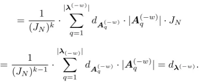
2. dλ=dλ(−w) andvλ=vλ(−w).
Proof. See Appendix A.
The theorem holds not only for a generic time lag w, but also for a set of r generic time lags
{w1, ..., wr}, with r >1.
We now introduce the important concept ofε-active time lag.
Definition 18. Given ε ∈ [0,1] and w ∈ {1, . . . , k}, a time lag w is said ε-active when, for any az∈A, the following conditions are fulfilled:
• |P(az|ai)−P(az|aj)|< ε, where ai can differ fromaj in all times but t−w, for any couple i, j,
• ε is the lowest number satisfying the previous inequality.
In other words, the observation of the process int−wbrings a “key information” to determine its evolution at timet.
This definition can be extended to combinations of severalε-active time lags as follows:
Definition 19. Given ε∈[0,1]and ρindexes w1, . . . , wρ ∈ {1, ..., k}, the time lagsw1, . . . , wρ are
said joint ε-active when, for any az ∈A, the following conditions are fulfilled:
• |P(az|ai)−P(az|aj)|< ε, whereai can differ fromaj in all times but t−w1, . . . , t−wρ, for
any couplei, j,
• ε is the lowest number satisfying the previous inequality.
Remark 20. It does not make sense to extend the search for activeρ-tuples whose size is greater than k−1, wherek is the order of the Markov chain {X(t), t≥0}. Verifying that all the k time lags areε-active is equivalent to find that none time is of particular importance over the others for
We now see how we can jointly use the definitions of longest-memory k and joint ε-active time
lags. Consider the time lags which are less than or equal to the longest-memory k, i.e. the set
{1, ...,lm-kλ}. If we know which time lags in{1, ...,lm-kλ}arejoint ε-active, we can neglect all the others and avoid to evaluate the corresponding partitions.
To be more precise, we detail here the conditions for selecting the non-dominated solutions and build
the efficient frontier. Such definitions will turn out to be useful in the next section, devoted to the
application of our methodology.
Definition 21. Let us consider a couple of partitions λu,λx ∈ Λ
k; we say that λu is d-m
-non-dominated (v-m-non-dominated) byλx when
dλu ≥dλx mλu ≥mλx
or
dλu ≤dλx mλu ≤mλx
(21)
vλu ≥vλx mλu ≥mλx
or
vλu ≤vλx mλu ≤mλx
.
According to the previous definition, dominated partitions will be discarded in our analysis; basically,
the rejected partitions show no lower distance (dλ, orvλ) and no higher multiplicity (mλ), with at
least a strict inequality holding.
We now turn to the optimization problems (19) and (20) and introduce the efficient frontier, defined
as follows:
Definition 22. Considerk¯∈ {1, . . . , N}.
i. The efficient frontierFm,d,¯k related to optimization problem (19) is:
Fm,d,¯k:=
∪
γ∈[0,1]
{(mλ∗, dλ∗)∈[0,1]×[0,2]},
where λ∗ is the solution of the problem:
min
λ∈Λk¯
dλ
s.t. mλ≥γ.
ii. The efficient frontierFm,v,¯k related to optimization problem (20) is:
Fm,v,¯k:=
∪
γ∈[0,1]
{(mλ∗, vλ∗)∈[0,1]×[0,0.25]},
where λ∗ is the solution of the problem:
min
λ∈Λk¯
vλ
It is worth noting that we can build an efficient frontier for each value ofk∈ {1, . . . , N}. In practice, once khas been set equal to ¯k, the procedure to build the efficient frontiers associated to the two
optimization problems (19) and (20) can be synthesized in the following points:
1. initially the researcher orders the set of admissible solutions by increasing values of their
distance indicator (vor d);
2. starting from the solution with the lowest value of distance, she/he scans for the next solution
with a higher distance and a higher value of multiplicity (m) and discards the intermediate
solutions (dominated in the sense of Definition 21);
3. step 2. is repeated until the worst value of distance is reached.
The partitions remaining after step 3. constitute the optimal solutions and the values of their
distance indicator and multiplicity measure represent theefficient frontier Fm,d,¯k orFm,v,¯k.
It is relevant to assess the finite time performance of the above 3 step procedure. Firstly, we stress
that the procedure provides the solution of the optimization problems (19) and (20) as the parameter
γvaries in [0,1]. The complexity of the problems increases dramatically as the number of time lags
and states of the Markov chain grow. The following result formalizes this aspect.
Proposition 23. The time required to span the set of admissible solutions is O([J2
NB(JN)]k
) for
optimization problem (19) andO([JNB(JN)]k
)
for optimization problem (20) asJN →+∞, where JN is the number of states and kis the order of a Markov chain.
Proof. See Appendix A.
As an example, Table 1 shows the cardinality of the set of admissible solutions for various
combina-tions of time lagskand statesJN characterizing a Markov chain. Remember that such cardinality
is equal to [B(JN)]k (see footnote 1).
Insert Table 1 here
6
Numerical Test
To test the effectiveness of our method, we devise the following experiment:
1. we consider a Markov chain of order k, with kset to a chosen value ¯k, and artificially design
the associated ¯k-path transition probability matrix. The rows on this matrix are joined
fol-lowing a partition, which we call here as “true” partition, where only some of the time lags
are “active” and equivalent states (i.e. those generating similar transition probabilities) are
grouped together. This matrix defines the effective conditional probability distribution of a
2. based on such matrix, we generate a simulated trajectory of 5,000 observations;
3. an empirical transition probability matrix is then estimated from this simulated series;
4. our optimization procedure is then applied both to the benchmark and to the empirical matrices
and their solutions (represented through efficient frontiers) are compared. Such procedure is
replicated for both the two distance indicators analyzed here.
If the procedure is effective, then the benchmark and the empirical solutions should “largely”
inter-sect and the true partition should be one of the preferred solutions. More specifically, our experiment
consists in a severe reverse-engineering test, where some parameter estimates obtained from
empir-ical investigation, instead of being tested for statistempir-ical significance, are compared with their “true”
values, which is a definitely more conclusive result. We also expect that the method should be fairly
robust to the choice of the distance indicator adopted.
We run this experiment starting with two different transition probability matrices.
6.1
k
-path transition probability matrix design
The considered Markov chains (and their transition probability matrices) are defined as follows:
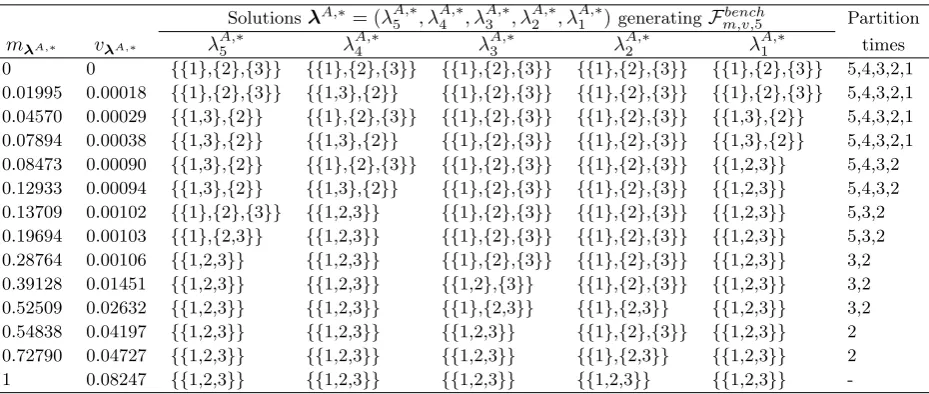
I. a Markov chain of order ¯k= 5 and with state spaceA={1,2,3}, such that only time lags 3 and 2 are active in the sense of Definition 18. This means that the values observed in time lag 1,
4, and 5 have no influence on the evolution of the process. So for comparison purposes we will
consider transition probability matrices Abench andAempir with dimensions 35
×3 = 243×3;
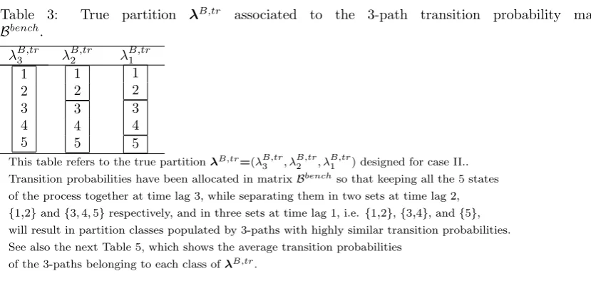
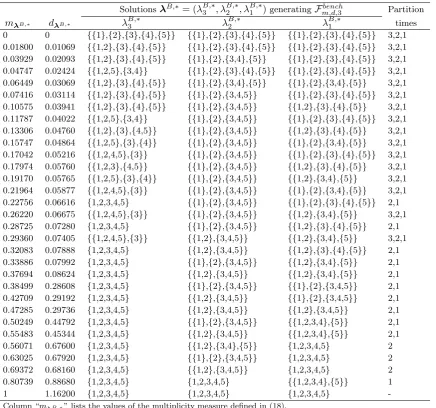
II. a Markov chain of order ¯k= 3 and with state spaceB ={1,2,3,4,5}, such that only time lag 2 and 1 are active. In this case, the transition probability matrices are denoted with Bbench andBempir and have dimension 53×5 = 125×5.
The four transition probability matrices are available at the web pagehttp://chiara.eco.unibs.
it/~pelizcri/CuttedTable1andTable2new.xls. To obtain a complete view of the information
embedded in these matrices, consider Tables 2 and 3, where the true partitions are clearly
repre-sented. We call these two partitions asλA,tr andλB,tr respectively for casesI. andII.. The same tables also show which time lags are “active”:
• time lags 3 and 2 in matrix Abench are joint 0.23-active (singularly considered,t−5, t−4, t−3,t−2, andt−1 areε-active, withεbetween 0.83 and 0.84);
• time lags 2 and 1 in matrix Bbench are joint 0.04-active (singularly considered, t
−3, t−2, andt−1 are 0.44-active, 0.34-active, and 0.39-active, respectively).
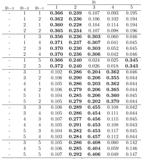
Tables 4 and 5 show the average values of the transition probabilities associated to the states
grouped following the true partitions. The black horizontal lines in the matrices help to represent
the corresponding classes. These partitions are formed combining the classes defined in each time
lag, as it has been discussed in the theoretical settings (see Section 3). Values are taken averaging
over the nonε-active time lags. In particular in Table 4, which refers to caseI., each row represents a 5-path observed at active time lags 2 and 3, and the transition probabilities are obtained averaging
27 rows (i.e. the combinations of 3 states in the 3 nonε-active lags) of matrixAbench. The rows in Table 5, which refers to caseII., are the average probabilities calculated over the corresponding 5 rows in matrixBbench(i.e. the 5 states in the only non ε-active time lag 3).
Insert Tables 4 and 5 here
Numbers in bold help to represent which states the process tends to evolve to preferably, conditional
on its past values. As it is immediate to observe, the rows tend to be very similar when they are in
the same group and change significantly from class to class.
6.2
Simulation and estimation of the empirical transition probability
ma-trix
As anticipated at the beginning of the present section, for each case a simulated trajectory has been
generated consisting of 5,000 values. The simulation has been based on a Monte Carlo method3. For
each simulated series the corresponding empirical transition probability matrix has been estimated,
based on the usual conditional frequency calculation.
The most obvious differences between the benchmark and the empirical matrices are concerned with
the values of the transition probabilities. Besides, another possible difference consists of the loss of
some rows in the empirical matrix, a case which can verify if the process has very low probabilities
(if not zero) to follow some paths. Finally some paths can be observed with a frequency which is too
low to supply a significant estimate of the corresponding row. To estimation purposes, rows with a
low frequency (i.e. less than 20) have been treated in the same way as the rows which have never
been observed in the simulated series: in both cases those rows have been set to zero, following (3).
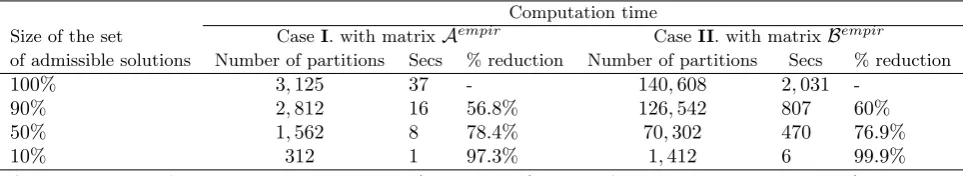
6.3
Optimization procedure
The set of admissible solutions in caseI. is formed by 3,125 partitions (the set of partitions onAis ΛA, with|ΛA|= 5, and|(ΛA)5|=|ΛA|5= 55). For case II. the same calculation results in 140,608
partitions (the set of partitions onB is ΛB, with|ΛB|= 52, and|(ΛB)3|=|ΛB|3= 523).
3
To solve the two optimization problems (19) and (20), we have calculated the distance indicators
and the multiplicity measure for every partition (see (14), (16), and (18)) in the set of admissible
solutions of casesI. andII.. For each case the procedure has been applied both to the benchmark and the empirical transition probability matrices. Summing up the combinations, the 3 step procedure
presented at the end of Section 5 has been applied 8 times (2 distance indicators × 2 cases × 2 transition probability matrices) and has generated 8 efficient frontiers Fbench
m,d,5, Fm,v,bench5, Fm,d,bench3,
Fbench
m,v,3,Fm,d,empir5,F
empir
m,v,5,Fm,d,empir3, andF
empir m,v,3.
Table 6 shows the time required to calculate the distance indicators and the multiplicity measure for
each case and both the benchmark and empirical transition probability matrices. The calculation
has been performed on a machine with an Intel Pentium M-processor at 2.8 Ghz.
Insert Table 6 here
6.4
Analysis of results
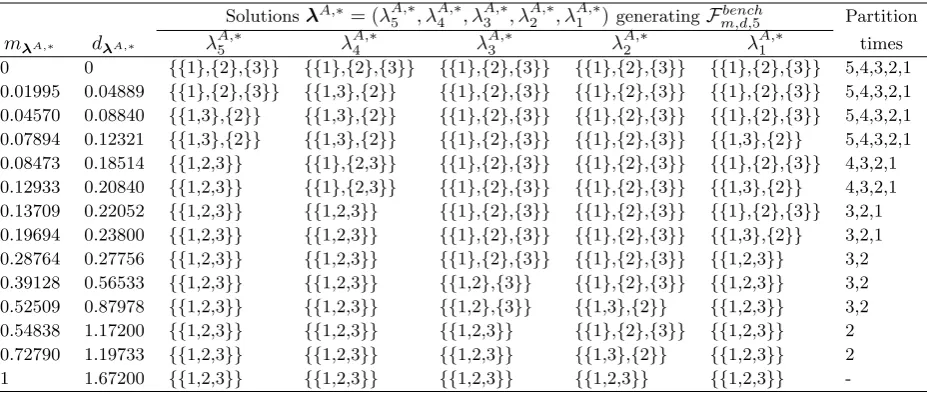
Tables 7, 8, 9, and 10 give details of the benchmark efficient frontiers calculated on the
bench-mark matrices for the two distance indicators and the two cases (i.e. Fbench
m,d,5, Fm,v,bench5, Fm,d,bench3, and
Fbench
m,v,3). It is interesting to analyze these results moving from the partition of singletons to the
all-comprehensive set partition. As more classes are aggregated the multiplicity indicator improves
at the price of increasing the distance indicator. This is no surprise, but it is important to analyze
the size of the increments in the two indicators passing from one point to the next on these frontiers.
Indeed it is possible to observe that the true partitions λA,tr and λB,tr represent a kind of
“cor-ner point” in each case. Before these key points the increase in the multiplicity measure is paired
with small increments of the distance indicators. On the contrary, after those turning points every
increase in the multiplicity tends to come at a price of a consistent increase in the distance.
Insert Tables 7, 8, 9, and 10 here
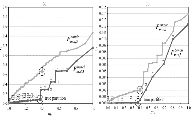
The previous arguments become even more evident observing Fig. 1 and Fig. 2, where the
bench-mark efficient frontiers are graphically represented for casesI. andII. respectively. Each figure has two panels, i.e. (a) and (b), corresponding respectively to the two optimization problems (19) and
(20). Partitions λA,tr and λB,tr separate the corresponding benchmark efficient frontiers (
Fbench m,d,5,
Fbench
m,v,5,Fm,d,bench3, and Fm,v,bench3) in two clearly different parts.
It is also possible to observe that in both cases the partitions generating the benchmark efficient
frontiers show partition times (see Definition 14) mainly coinciding with theε−active times.
Insert Figures 1 and 2 here
Turning to the analysis of the empirical efficient frontiers (Fm,d,empir5,Fm,v,empir5,F
empir m,d,3, andF
empir m,v,3), in