Estimating Semiparametric Panel Data
Models by Marginal Integration
Qian, Junhui and Wang, Le
Shanghai Jiao Tong University
10 November 2009
Online at
https://mpra.ub.uni-muenchen.de/18850/
by Marginal Integration
1Junhui Qian School of Economics Shanghai Jiao Tong University
Fua Hua Zhen Road 535 Shanghai, 200052, China
Le Wang
University of New Hampshire 15 College Road Durham, NH 03824
Abstract
We propose a new methodology for estimating semiparametric panel data mod-els, with a primary focus on the nonparametric component. We eliminate indi-vidual effects using first differencing transformation and estimate the unknown function by marginal integration. We extend our methodology to treat panel data models with both individual and time effects. And we characterize the asymptotic behavior of our estimators. Monte Carlo simulations show that our estimator behaves well in finite samples in both random effects and fixed effects settings.
This version: November 10, 2009
JEL classification codes: C13; C14; C24
Key words: Semiparametric Panel Data Model, Partially Linear, First Differencing, Marginal Integration
1
1. Introduction
In many empirical studies involving panel data sets, at least in the initial stage of research,
it is useful to consider semiparametric models like the following,
Yit=αi+β′Zit+f(Xit) +εit, (1)
whereαi is unobserved individual effect andXit is most likely a low-dimensional covariate
vector that relates to Yit via an unknown function f. We call the above model
semipara-metric since only part of the covariate vector (i.e., Zit) is parameterized; and since the
unknown functionf is in general nonlinear, the above model is also called a partially linear panel data model. As a middle course between parametric and nonparametric extremes,
semiparametric models are very appealing for its flexibility to balance between precision
and robustness.
On some occasions, the nonparametric component f(Xit) is treated as a nuisance term
and the functional form f need not be estimated. This may be reasonable if Xit only
performs a “controlling” role and there is little ambiguity toward the relationship between
the variables of interest. However, ifXitare indeed among the variables of interest, and when
the theoretical predictions regarding the relationship between Xit and Yit are ambiguous
or controversial, the estimation of f may become the central objective. For example, the classical research on Kuznets curve that investigates the relationship between income and
inequality centers on the estimation of a nonlinear (supposedly inverted-U shape) function
(See, e.g., Banerjee and Duflo (2003)). This is also true with the recent literature on
environmental Kuznets curve which examines the relationship between income and pollution
level (See, e.g., Millimet, List, and Stengos (2003)). Other important empirical topics such
as the estimation of the Engel curve, production function, earnings-age profile, and so
on, also boil down to estimating a possibly nonlinear relationship between two economic
may not be the end of analysis. But even as an initial analysis before parameterization, a
robust and reasonably accurate estimation of the nonlinear component is essential for the
success of future modeling and analysis.
In recent years, indeed, a lot of research has been done in estimating semiparametric
panel data models, the nonlinear component treated as a term of interest. As in the case
of linear panel data models, these efforts can be largely grouped into three categories, RE
(Random Effects), FE (Fixed Effects), and FD (First Differencing), depending on how they
treat the unobserved effects.
The RE school treats the unobserved effects as exogenous and puts them into the
resid-ual. Li and Stengos (1996), following Robinson (1988), develop a root-N consistent IV estimator for the estimation of β, assuming that αi is uncorrelated with other covariates.
Although their focus is on the linear part, the nonlinear part can be easily estimated using
a second-stage kernel regression. This simple approach, which we may call the pooled
esti-mation, does not take into account the special covariance structure of the composite error,
αi+εit. However, Ruckstuhl, Welsh, and Carroll (2000) show that the pooled estimator has
better asymptotic properties than the quasi-likelihood estimator which takes into account
the covariance structure. Ruckstuhl, Welsh, and Carroll (2000) propose an alternative
two-step estimator, which we may call LL-RE (Local Linear Random Effects) estimator, that
also accounts for the covariance structure. They show that LL-RE may achieve smaller
asymptotic variance than the pooled estimator does, but the bias is in general
incompa-rable. Recently Su and Ullah (2007) generalize the two-step estimator to the multivariate
case.
As in linear panel data models, the FE approach treats the unobserved effects as dummy
variables. Su and Ullah (2006) propose to estimate the nonlinear component by profile
likelihood estimation, which boils down to a locally linear kernel smoothing, controlling
for fixed effects by dummies. To use the usual panel data terminology, the estimator by
Variables) estimator. Recently, Mammen, Støve, and Tjøstheim (2009) develop an iterative
procedure based on smooth backfitting algorithm for estimating additive panel data models,
treating unobserved effects as dummy variables. Their procedure may be directly applied
to semiparametric panel data models with fixed effects.
Finally, the FD approach imposes no assumptions on unobserved effects and eliminates
unobserved effects by first differencing. However, this transformation leaves us a structure
of the following form, m(Xit, Xi,t−1) =f(Xit)−f(Xi,t−1), making the recovery of f
diffi-cult, even after successful estimation of the linear part. Henderson, Carroll, and Li (2008)
solve this problem by using an iterative backfitting procedure based on the first-order
con-dition of a profile likelihood criterion. Alternatively, Lee and Mukherjee (2008) propose to
first approximatef using a local Taylor series expansion before taking first differencing (or, alternatively, within transformation). However, the function itself is eliminated from
con-sideration by first differencing, and hence their approach deals only with the first derivative
of f.
In this paper we propose a noniterative method that is based on marginal integration.
We observe thatm(u, v) is an additive function and that marginal integration of an estimate of m recovers f. The technique of marginal integration, under the name of “projection”, is introduced by Auestad and Tjøsstheim (1991) in the context of time series regression.
A more systematic treatment is given in Tjøsstheim and Auestad (1994). This method
is independently invented by Newey (1994) and Linton and Nielsen (1995) in the context
of i.i.d. cross-section regression. Linton and H¨ardle (1996) generalize the method to deal
with additive regression with known links. For important developments of this technique,
see Masry and Tjøsstheim (1997), Linton (1997), Fan, H¨ardle, and Mammen (1998), Kim,
Linton, and Hengartner (1999), Cai and Masry (2000), and Hengartner and Sperlich (2005).
The estimator we develop is conceptually simple, hence it is straightforward to analyze
its statistical properties. Indeed, we derive the asymptotic distribution of our estimator
the computational procedure for our estimator is noniterative, hence it is easy to
imple-ment in practice and also fast enough for finite sample investigations using Monte Carlo
simulations. The disadvantage of our approach, however, is some efficiency loss during the
unconstrained nonparametric estimation of m(u, v). In particular, the information in the antisymmetric structure ofm(u, v) is lost. As a preliminary attempt, we propose a sample augmentation technique to make use of the structure. Although simulation results indicate
some success for this technique, we are currently unable to validate it theoretically. Hence
our asymptotic theory does not rely on sample augmentation.
The rest of the paper is organized as follows. The next section presents the model,
describes our methodology, and gives asymptotic properties of our estimators. We first
consider panel data models with only individual effects, then we extend our methodology
to treat two-way effects models. Section 3 presents some Monte Carlo evidence on how our
estimator behaves in the finite sample setting. All mathematical proofs are provided in the
appendix.
2. The Model and Estimation
We consider the semiparametric (partially linear) panel data model in (1) which is
repro-duced here for convenience,
Yit=αi+β′Zit+f(Xit) +εit, i= 1,· · ·, N, t= 0,1,· · · , T, (2)
where β ∈ Rb, Zit ∈ Rb, Xit ∈ Rd, and all other variables are scalars. f is an unknown
d-dimensional smooth function. Some or all elements inZitmay be correlated with residual
εit. And we allow for arbitrary correlation between the unobservable individual effectαi and
the regressors (Xit, Zit). The individual effect may be called fixed effect if it is correlated
to avoid, and the fact that it is extremely difficult to interpret f ifd≥4.
One extension to the model in (2) is to introduce a time effect into the original model.
The extended model, called two-way effects (individual and time effects) model, will be
discussed later in the paper.
To estimate the model, we first take the FD (First Differencing) transformation of (2)
across time tfor each groupi,
∆Yit=β′∆Zit+f(Xit)−f(Xi,t−1) +eit, i= 1,· · · , N, t= 1,· · · , T, (3)
where ∆Yit =Yit−Yi,t−1, ∆Zit=Zit−Zi,t−1, andeit=εit−εi,t−1. This first-differencing
transformation eliminates the individual effects αi. Throughout the paper, we assume:
Assumptions A
(1) (Xit, Zit, eit) are i.i.d. ini.
(2) For eachi,Xitis strictly stationary with a well defined densitypon a compact support
C∈Rd; and the marginal and joint densities ofXitare bounded from above and from
zero.
(3) eitis independent of (Xit), andE(eit) = 0,E(eit2) =σ2t,E|eit|4+ǫ<∞for some ǫ >0.
A(1) is fairly standard for panel data models. The stationarity assumption in A(2) is
stronger than necessary and is made for simplifying analysis. We may obtain similar
asymp-totic results if we assume that (Xit, Xi,t−1) admits a joint density that does not vary over
t, which is not sufficient for stationarity. A(3) is fairly weak, allowing for serial correlation inεit. Indeed, our methodology works best if εit is a random walk. Finally, note that the
covariance matrix of ei = (ei1, ..., eiT)′ is non-diagonal in general. Later in this section,
we will discuss possibilities of using this fact to improve efficiency. We now turn to the
2.1 The Linear Component
For the linear part parameterized by β, the transformed model in (3) is a special case of the model considered in Li and Stengos (1996). Let u = (u1, ..., ud)′ and v = (v1, ..., vd)′,
and letp2(u, v) be the joint density of (Xit, Xi,t−1). The model in (3) implies
Yit∗=β′Zit∗ +uit,
where Y∗
it = ρit(∆Yit−E(∆Yit|Xit, Xi,t−1)), Zit∗ = ρit(∆Zit−E(∆Zit|Xit, Xi,t−1)), uit =
ρiteit, and ρit = p2(Xit, Xi,t−1). Working with this density weighted equation enables
us to avoid the random denominator problem typical in nonparametric kernel regression
estimation.
Assuming there exists a vector of instrumental variables Wit ∈ Rb, we may construct
an IV estimator forβ. Let Wit∗ =ρit(Wit−E(Wit|Xit, Xi,t−1)). And let the capital letters
without subscripts denote the matrices of observations of the corresponding variable. More
specifically, we denote Zi = (Zi1, ..., ZiT)′ andZ ≡(Z1′, ..., ZN′ )′. Throughout the paper we
use the same matrixization and denoteZ = [Z′
it]. Then we have an infeasible IV estimator
ˆ
β = (W∗′Z∗)−1W∗′Y∗,assuming that the term in parentheses is invertible.
To make the IV estimator feasible, we estimate ρit by ˆρit = 1/(N T))PjsLg(Xit−
Xjs)Lg(Xi,t−1−Xj,s−1), whereLg(u) =g−dQdj=1l(uj/g),l is a univariate kernel and g is
the associated bandwidth. The conditional means are estimated by 1/(N T)PjsξitLg(Xit−
Xjs)Lg(Xi,t−1−Xj,s−1), whereξit denotes ∆Yit, ∆Zit, and Wit. Assuming that ˆW∗′Zˆ∗ is
invertible, we obtain the following feasible IV estimator,
ˆ
β = ( ˆW∗′Zˆ∗)−1Wˆ∗′Yˆ∗. (4)
Let the class of kernels Kν and the function class Gςα be defined as Definition 1 and
Definition 2 of Robinson (1988), respectively. Kernels inKν are of orderν, and the functions
inGα
the moment properties of the remainder. In particular, the functions in G∞
ς are bounded.
For the root-N consistent estimation ofβ, we adapt the following assumptions from Li and Stengos (1996),
Assumptions B
(1) p2 ∈ Gς∞for some constantς ≥1,f ∈ Gν4+ǫ,E(∆Zit|Xit, Xi,t−1)∈ Gν4+ǫ for someǫ >0
and positive integerν withς < ν ≤ς+ 1.
(2) There exists an IV vector Wit ∈ Rb such that Wit is i.i.d. in i, E(Wit4+ǫ) < ∞,
E(Wit|Xit, Xi,t−1)∈ Gν4+ǫ, andE(eit|Wit) = 0 for all t. And Ξ =EW12∗Z12∗ ′ is
nonsin-gular.
(3) l∈ Kν, and as N → ∞,a→0, andN a4d→ ∞, and N a4ν →0.
The assumptions in B(2) are fairly standard for an IV vector. For a typical application
withd= 1, B(3) is satisfied if we letν = 2 and choose a second-order kernel for l. B(1) is satisfied ifp2 has continuous partial derivatives andf is twice continuously differentiable. If
d >1, then we have to use a higher order kernel forlandf needs to have more derivatives, which is one form of the curse of dimensionality.
The assumption onp2, which states that p2 is bounded and at least first-order partially
differentiable with a Lipschitz-continuous remainder, is stronger than that is made in Li and
Stengos (1996), who only require Lipschitz continuity. This stronger assumption is made
for estimating the nonlinear part and is not required for the following theorem, which is
proved in Li and Stengos (1996).
Theorem 1. Under assumptions A and B, we have
√
where Ψ = 1/T2PtPsE(e1te1sW1t∗W1s∗′). Furthermore, we can consistently estimate Ψ
and Ξ by plugging in the estimates for each term.
2.2 The Nonlinear Component
The major contribution of this paper is in estimating the unobserved function f(·). To simplify the notations, we denoteRit= ∆Yit−β′∆Zit. We rewrite (3) as
Rit=m(Xit, Xi,t−1) +eit, i= 1,· · · , N, t= 1,· · ·, T, (6)
wherem:R2d→R is an additive function:
m(u, v) =f(u)−f(v), u, v∈Rd. (7)
Obviously,m(u, v) =−m(v, u). Hence m(u, v) is antisymmetric.
We may easily estimate m(u, v) using multivariate kernel smoothing methods. The popular estimators are Nadaraya-Watson (Nadaraya (1964); Watson (1964)), Gasser-M¨uller
(Gasser and M¨uller (1984)), and local linear (Stone (1977); Cleveland (1979); Fan (1992);
Ruppert and Wand (1994)), among others. In principle, each of these approaches would
serve our purpose. We will prove asymptotic properties only for the local linear method,
which includes Nadaraya-Watson as a special case.
LetK(u) =Qdi=1k(ui), wherekis a univariate second-order symmetric kernel. And
de-noteKH(u) =|H|−1K(H−1u), whereH = diag(h1, ..., hd) is a diagonal bandwidth matrix.
The local linear estimator ofm(u, v) solves the following problem for α,
min
α,γ1,γ2 N
X
i=1 T
X
t=1
£
Rit−α−γ1′(Xit−u)−γ′2(Xi,t−1−v)¤KH(Xit−u)KH(Xi,t−1−v). (8)
It is well known that the problem in (8) is a weighted least square problem. LetR = [Rit]
u)KH(Xi,t−1−v)]. Note that we suppress the dependence onuandvof Γ andW. Assuming
that Γ′WΓ is invertible, (8) has a solution for ˆα (hence ˆm(u, v)),
ˆ
m(u, v) = ˆα=ι′(Γ′WΓ)−1Γ′W R, (9)
where ι= (1,
2d
z }| {
0, ...,0)′. Note that ˆγ
1 supplies an estimate of ∂f∂u(u). If our primary goal is
estimating the partial derivatives, we may stop here. While it is possible to recoverf up to an additive constant from partial derivatives by numerical integration, we are obviously not
satisfied with this solution; the reason is that although the asymptotic properties of ˆγ(u) are well known, those ofRxˆγ(u)duare not. And it is conjectured that statistical error may accumulate through numerical integration. We focus on ˆm(u, v), which is the stepstone for estimatingf.
We proceed to estimate f(·) by marginally integrating ˆm(u, v),
ˆ
f(u) =
Z
C
ˆ
m(u, v)q(v)dv, (10)
whereq is a predetermined density function. For model identification, we follow Hengartner and Sperlich (2005) and assume RCf(u)q(u)du = 0. Note that this condition reduces to
E(f(Xit)) = 0 as in Linton and H¨ardle (1996) if we takeq=p. It is easy to see the rationale
behind (10),
Z
C
m(u, v)q(v)dv=
Z
C
(f(u)−f(v))q(v)dv =f(u).
Note that, in practice, it is not always necessary to impose the identification condition. If
the condition does not hold,f can still be identified up to an additive constant.
We may implement the marginal integration in (10) by numerical integration methods
such as Simpson’s or Trapezoidal rules. Let the number of evaluation points on each
O(N) operations. This may become a practical concern and calls for discretion over the balance between numerical accuracy and computational time.
An alternative method of calculating the marginal integration is to generate i.i.d.
sam-ples (X∗
k,k= 1, ..., n) from the distributionq and to construct ˆfmc(u) = 1nPnk=1mˆ(u, Xk∗).
If n is large enough, ˆfmc approximates ˆf well. We may well choose q(·) to be the density
function of Xi,t. In this case we may use the sample version of (10),
ˆ
fs(u) = 1
N(T + 1)
N
X
i=1 T
X
t=0
ˆ
m(u, Xi,t). (11)
Asymptotically, this estimator behaves the same as (10) when q is the density of Xi,t. We
assume:
Assumptions C
(1) qis a bounded density function, defined on the compact supportC, twice continuously differentiable, and RCf(u)q(u) = 0.
(2) k is a second-order kernel that is positive, bounded, symmetric, and defined on the support C.
(3) H = H0N−1/(4+d), where H0 is a diagonal matrix with positive constants on the
diagonal.
These assumptions are fairly standard in literature. Let ˆf be defined as in (10). And denote
ϕ(k) =R k(u)2du, µ2(k) =R u2k(u)du, Df = ∂f∂u, andHf = ∂ 2
f
∂u∂u′. The following theorem
is the major result of this paper.
Theorem 2. Letube an interior point of supp(p) and let Assumptions A, B, and C hold. Given a fixed T and as N → ∞, we have
where
B(u) = 1 2µ2(k)
·
tr¡H02Hf(u)
¢ −
Z
C
tr¡H02Hf(v)
¢
q(v)dv
¸
, (13)
and
V(u) = ϕ
d(k)¯σ2
T|H0|
µZ
C
q2(v)
p2(u, v)
dv
, (14)
where ¯σ2 = 1/TPtσ2t.
The proof is given in the Appendix. Here we make a number of remarks.
Remark 1: If we impose i.i.d. condition onXitacrosstas well asi, and if we takeq=p,
the asymptotic variance would take an even simpler form:
V(u) = ϕ
d(k)¯σ2
T|H0|p(u)
.
Remark 2: We may consistently estimateV(u) by
ˆ
V(u) =N−2(2+d)/(4+d)T−2
N X i=1 T X t=1 ˆ
e2itθˆ2it, (15)
where ˆθit= 1/n˜Pj=1n˜ wj(u, Xj∗) with
wj(u, Xj∗) =
KH(u−Xit)KH(Xj∗−Xi,t−1)
PN i=1
PT
t=1KH(u−Xit)KH(Xj∗−Xi,t−1)
,
where (X∗
j, j = 1, ...,n˜) are drawn from the distribution with densityq. Ifq =p, we may
simply use (Xit) in place of (Xj∗).
Remark 3: We can construct confidence bands forf using the asymptotic result. Denot-ing the (1− a2) quantile of the standard normal distribution with z1−a
confidence bands,
"
ˆ
f(u)−N−2/5¡B(u) +z1−a
2V
1/2(u)¢, fˆ(u)
−N−2/5¡B(u)−z1−a
2V
1/2(u)¢
#
.
With some under-smoothing (i.e.,h=o(N−1/5)), we may ignore the bias term and use only
the asymptotic variance to construct confidence bands forf(u). At the cost of computation time, we may also improve the quality of confidence bands by bootstrap. See H¨ardle and
Marron (1991) for more details.
Remark 4: An optimal H0 may be found by minimizing AMISE (Asymptotic Mean
Integrated Squared Error). This is best illustrated by considering the case of d= 1, when
H0=h0 is a positive scalar. We minimize
AMISE(h0) =
Z
C
¡
B2(u) +V(u)¢du.
Then we obtain an optimalh0:
h0 =
µ
ϕ(k)¯σ2 µ22(k)T
ϑ2
ϑ1
¶1 5
,
where
ϑ1 =
Z
C
(f′′(u)−
Z
C
f′′(v)dv)2du, and ϑ2=
Z
C
Z
C
q2(v)p−21(u, v)dudv.
Replacing the unknown quantities (¯σ2,ϑ1, andϑ2) with their estimates, we obtain a plug-in
bandwidth selector. And the above strategy can be easily extended to multivariate case.
We may also choose bandwidths using delete-one CV (Cross-Validation), generalized
CV (Craven and Wabha, 1979), or model selection procedures such as Mallows’(1973) Cp
and CL procedures. See Li (1987) and Andrews (1991) for the asymptotic properties of
Remark 5: If the Nadaraya-Watson kernel smoothing is used for estimatingm(u, v), the asymptotic variance of ˆf(u) would be the same as in (14), but the asymptotic bias takes the following form:
B(u) = µ2(k)
·
1 2tr
¡
H02Hf(u)¢−
1 2
Z
C
tr¡H02Hf(v)¢q(v)dv
+D′f(u)H02
Z
∂log(p2(u, v))
∂u q(v)dv− D
′ f(v)H02
Z
∂log(p2(u, v))
∂v q(v)dv
¸
.
Remark 6: If f is twice partially differentiable, our estimator achieves the best conver-gence rate possible. However, we require higher-order differentiability of f to estimate the linear component if d≥2. Recall that in Assumption B, we require f ∈ Gν4+ǫ and ν > d. The optimal rate is thus N−ν/(2ν+d), higher than our estimator achieves. To achieve the
optimal rate, we need higher-order locally polynomial smoothing to reduce bias. We choose
not to do so for the attractive properties of local linear estimators (Fan and Gijbels (1992),
Ruppert and Wand (1994)). And if there is no linear part, we only need twice
differentiabil-ity forf, regardless ofd. Then the optimal rate of kernel regression estimator isN−2/(4+d),
which is achieved by our estimator.
Remark 7: Finally, the form of the asymptotic varianceV(u) suggests when our method might fail. That is when Xit is accurately predictable by Xi,t−1. In this case, if we write
p2(u, v) = p(u|v)p(v), p(u|v) would be close to zero except in a small neighborhood of v,
hence a largeV(u). This happens, for example, ifXit is highly persistent in t.
2.3 Efficiency Issues
Now we discuss two issues related with the efficiency of our estimator. The first is concerned
with how we may use the covariance matrix of ei = (ei1, ..., eiT)′, which is in general not
diagonal. The second issue is concerned with how we may use the antisymmetric property
Covariance Structure
Let Σ denote the covariance matrix ofei, which is diagonal only whenεit is a random walk.
Indeed, ifεit is i.i.d. acrosst, Σ would be a tridiagonal matrix with 2’s on the main diagonal
and -1’s on the sub-diagonal. Our estimator ofm(u, v) does not make use of this structure, and therefore it is possible to be improved.
One way to take advantage of the covariance structure is to estimate m(u, v) by the quasi-likelihood method proposed by Severini and Staniswalis (1994). The quasi-likelihood
estimator of m(u, v) is the intercept in the solution ofθ in
Γ′¡IN ⊗Σ−1¢ΓW(Y −Γθ) = 0,
whereIN is anN-dimensional identity matrix and⊗denotes Kronecker product.
We may also employ a two-stage procedure similar with Ruckstuhl, Welsh, and Carroll
(2000) and Su and Ullah (2007). Let ηit = (Xit, Xi,t−1) and ηi = (ηi1, ..., ηiT)′. The
two-stage estimator is based on the following identity
τΣ−12R i−
³
τΣ−12 −I T
´
M(ηi) =M(ηi) +τΣ− 1 2e
i,
whereτ is a positive constant, Ri = (Ri1, ..., Ri,T)′, andM(ηi) = (m(ηi1), ..., m(ηiT))′. The
first step obtains a local linear estimator of m (ignoring the covariance structure) and an estimator of Σ. Then we replace unknown quantities on the left with their estimates and
run a second-stage local linear regression.
It is not clear, however, that the above treatments may improve the accuracy of our
esti-mator. In a similar context, Ruckstuhl, Welsh, and Carroll (2000) show that the asymptotic
variance of the quasi-likelihood estimator is of higher order than that of the simple “pooled
estimator”, that is, the estimator ignoring covariance structure. The two-stage estimator
In explaining why the simple pooled estimator performs so well asymptotically, Ruckstuhl,
Welsh, and Carroll (2000) point out that the covariance structure is a global property of the
residual which may not be important for methods that act locally in the covariate space.
Sample Augmentation
The second issue is concerned with the structure ofm(u, v), which is by definition antisym-metric. We do not make use of this information in estimatingm(u, v) using unconstrained kernel smoothing methods. Hence our estimator suffers from some efficiency loss. One
way to impose the antisymmetric structure onm(u, v) is to generate another copy of data that is antisymmetric to the original data, and to use both the original data and their
antisymmetric mirror in kernel smoothing.
To see this, recall that for any triplet (Rit, Xi,t, Xi,t−1), we have
E(Rit|X) =f(Xi,t)−f(Xi,t−1),
sinceεit is assumed to be independent of X. Then the triplet (−Rit, Xi,t−1, Xi,t) must also
satisfy the above equation and can be included in the sample. We may call this practice
“sample augmentation”. However, our development of asymptotic theory does not extend
easily to the augmented sample, which obviously contains nonindependent (antisymmetric)
observations. Limited simulation results show that sample augmentation may considerably
improve our estimator. Undoubtedly it calls for further research into the general theory of
imposing prior structures on multivariate nonparametric estimation (not just the
antisym-metric structure in our case) by some type of sample augmentation.
2.4 Two-Way Effects Models
For some applications it is desirable to include a time effect in model (2), controlling for
two-way effects panel data model. To focus on the main idea, we consider the following simplified
model,
Yit =αi+φt+f(Xit) +εit, i= 0,1,· · ·, N, t= 0,1,· · ·, T, (16)
where (φt) represent time effects andXit is univariate2.
The model in (16) contains time effects (φt) that do not disappear with the first
dif-ferencing procedure described above. To eliminate φt, we take another difference across
individual ifor each timet. Thus we have
∆2Yit= [f(Xit)−f(Xi,t−1)−f(Xi−1,t) +f(Xi−1,t−1)] +eit, (17)
wherei= 1,· · ·, N,t= 1,· · ·, T, andeit=εit−εi,t−1−εi−1,t+εi−1,t−1. SettingRit= ∆2Yit
and v= (v1, v2, v3)′, we rewrite (17) as
Rit=m(Xit, Xi,t−1, Xi−1,t, Xi−1,t−1) +eit, i= 1,· · ·, N, t= 1,· · · , T, (18)
wherem:R4 →Ris an additive function that satisfies
m(u, v)≡m(u, v1, v2, v3) =f(u)−f(v1)−f(v2) +f(v3). (19)
We estimate m using local linear smoothing. The form of ˆm is the same as in (9), but the definition of each term should be modified. Let ˜N =N if N is even, else ˜N = (N −1)/2. We setι= (1,0,0,0,0)′. Γ is now a 5-column matrix [1,(X2i,t−u),(X2i,t−1−v1),(X2i−1,t−
v2),(X2i−1,t−1 −v3)]i=1,2,...,N ,t=1,2,...,T˜ . The diagonal elements of W are now kh(X2i,t −
u)kh(X2i,t−1−v1)kh(X2i−1,t−v2)kh(X2i−1,t−1 −v3), where kh(u) = k(u/h)/h and k is a
second-order symmetric kernel. Finally, R= [R2i,t].
Note that in these definitions we only use non-overlapped cross-sections. For example,
2
For a multivariateXit with dimensiond, our methodology would involve nonparametric estimation of a 4d-dimensional pilot function. The curse of dimensionality would render the two-way effects models with
we do not include [(X2i−1,t−u),(X2i−1,t−1 −v1),(X2i−2,t −v2),(X2i−2,t−1 −v3)] in the
definition of Γ. So in a sense we have dropped half of the sample. This is to deal with the
technical issue arising from the second differencing transformation across individuals. After
this transformation, the observationsUit ≡(Rit, Xit, Xi,t−1, Xi−1,t, Xi−1,t−1) are no longer
i.i.d. across i, making some of the well known asymptotic results of local linear estimators unapplicable. Undoubtedly this would affect the efficiency of the estimator and should not
be rigidly followed in practical applications.
We then estimatef(u) by
ˆ
f(u) =
Z
ˆ
m(u, v)q(v1)q(v2)q(v3)dv1dv2dv3, (20)
where q(v) is a predetermined univariate density function. As in the previous section, we may implement (20) by numerical integration or sample integration using actual or
simulated data.
Being 4-dimensional, m is endowed with a more complex structure of symmetry or antisymmetry. Specifically, we have
m(u, v1, v2, v3) = −m(v1, u, v3, v2),
m(u, v1, v2, v3) = −m(v2, v3, u, v1), and
m(u, v1, v2, v3) = m(v3, v2, v1, u).
We may again use this structural information for sample augmentation to improve efficiency.
For the development of asymptotic theory, we assume,
Assumptions D
(2) For eachi, all joint densities of (Xit) are continuously differentiable.
(3) kis a bounded and symmetric second order kernel onC.
(4) h=h0N˜−1/5, where h0 is a positive constant.
Let p4(u, v1, v2, v3) denote the joint density of (Xit, Xi,t−1, Xi−1,t, Xi−1,t−1). The following
theorem gives the asymptotic properties of the estimator ˆf defined in (20).
Theorem 3 Letu be an interior point of supp(p). If Assumptions A and D hold, then
˜
N2/5( ˆf(u)−f(u))→dN(B(u), V(u)), (21)
where
B(u) = 1 2h
2 0µ2(k)
µ
f′′(u)−
Z
C
f′′(s)q(s)ds
, (22)
V(u) = ϕ(k)¯σ
2
h0T
µZ q2(v
1)q2(v2)q2(v3)
p4(u, v1, v2, v3)
dv1dv2dv3
(23)
The proof is a straightforward extension of the proof for Theorem 2 and hence omitted.
Note that, unlike the individual effect αi, the time effect φt can be consistently estimated,
assuming that φ0 = 0. Let ∆Yit = Yit −Yi,t−1 and ∆φt = φt−φt−1, t ≥ 1. We can
consistently estimate ∆φt by
d
∆φt=
1
N
N
X
i=1
(∆Yit−( ˆf(Xit)−fˆ(Xi,t−1)).
3. Simulations
In this section we use simulations to answer the following questions: does our estimator
random effects; (2) when (αi) are fixed effects; (3) and when (Xit) is persistent (but still
stationary) over time?
3.1 The Setup
We consider the following data generating process (DGP),
Yit =αi+f(Xit) +σεit, i= 1, ..., N, t= 1, ..., T, (24)
whereXit is a scalar random variable;εit is an i.i.d. N(0,1) random variable; andf(·) is a
pre-specified function to be estimated. And we experiment with two specifications ofαi,
(a) Random Effects (RE) : αi is i.i.d. N(0,4), independent of (Xit), which are i.i.d.
uniformly distributed between [−2,2].
(b) Fixed Effects (FE):αi is i.i.d. N(0,4) dependent on (Xit); the dependence is imposed
by generatingXitbyXit=αi/2+Uit, whereUitis i.i.d. uniformly distributed between
[−2,2].
We consider the following functional forms forf:
(1) f1(x) =−1/2x2,
(2) f2(x) =xcos(πx),
(3) f3(x) =x+ 2 exp(−16x2),
(4) f4(x) = sin(2x) + 2 exp(−16x2).
f1 is of inverted U shape, which is often seen in empirical economics. f2 is used in Linton
and Jacho-Cha´avez (2009), andf3 and f4 are used in Fan and Gijbels (1992). We use these
familiar functional forms to facilitate comparisons in literature. Throughout the simulations,
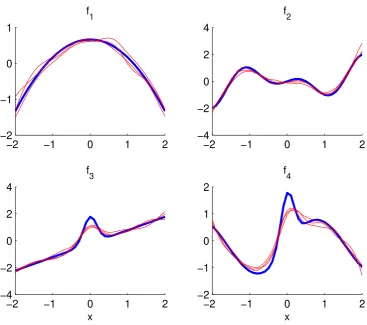
3.2 A Graphic Illustration
Figure 1 plots three consecutive FD estimates of each function. The estimated and the true
functions are shifted so that they all integrate to zero. We implement the FD estimator
using the sample version of marginal integration in (11) with the standard normal kernel.
We use the plug-in bandwidth described in Remark 4. And we choose T = 5 and N = 50, and takeαi to be random effects.
It can be seen that these estimates trace the true functions (bold solid lines) well, even
in locations near the boundary. Forf3 and f4, there is some under-smoothing in the bump
area. Recall that the plug-in bandwidth minimizes estimated AMISE, which is a global
distance metric. For functions such as f3 and f4, it may be better to use bandwidthh(x)
that is a function ofx and minimizes some local distance metric.
It should be noted that Figure 1 is only of illustrative purpose. We now turn to repeated
experiments for a more conclusive view of how our estimator performs in finite samples.
3.3 Comparative Performance
In the repeated experiments, we first compare our estimator with the estimator proposed in
Ruckstuhl, Welsh, and Carroll (2000) and Su and Ullah (2007), which works for the
random-effects specification; and that proposed in Su and Ullah (2006), which is designed for the
fixed-effects specification. As mentioned in the introduction, we may call the former method
LL-RE (Local Linear Random Effects) and the latter LL-LSDV (Local Linear LSDV). We
call our method FD (First Differencing).
We fixT = 5 and examine the finite sample performance of FD, LL-RE, and LL-LSDV when N is 50 and 100. We experiment with both low-noise level (σ = 0.5) and high-noise level (σ= 1). We do not impose identification condition in the simulations. Hencef is only identified up to an additive constant. We define the ISE (Integrated Square Error) of an
estimate ˆf by
ISEh( ˆf) =
Z
−2 −1 0 1 2 −2
−1 0 1
f 1
−2 −1 0 1 2
−4 −2 0 2 4
f 2
−2 −1 0 1 2
−4 −2 0 2 4
f 3
x
−2 −1 0 1 2
−2 −1 0 1 2
f 4
[image:23.595.133.501.202.527.2]x
Figure 1: An Illustration of FD Estimates. In each diagram, the bold line is the true function and the three thin lines are FD estimates from three random experiments. f1,f2,
wheref∗(x) =f(x)−Rb
af(x)dx/(b−a). f∗ is the true function shifted by a constant such
thatf∗integrates to zero. ˆf∗ is similarly defined. The ISE obviously depends on the choice
of bandwidth, hence the subscript. For better comparisons, we use a pre-specified set of
bandwidths. More specifically, we varyhfrom 0.1 to 0.6, with a small step size 0.03 within [0.1,0.25] and a bigger step size 0.05 in the remaining.
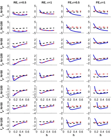
We repeat our experiment 500 times. Taking average of the ISEh, we obtain an MISEh
for each estimator. Figure 2 compares the logarithm of MISEh. The first two columns
correspond to RE experiments and the third and the fourth columns correspond to FE.
The first two rows correspond tof1, the third and the fourth rows correspond tof2, and so
on. The odd rows correspond to N = 50 and the even rows correspond to N = 100. The odd columns correspond toσ = 0.5 and the remaining columns correspond toσ= 1.
We make the following observations from Figure 2. First, overall, FD works well for
both RE and FE specifications. It can be seen that when the underlying DGP is RE, FD is
a close competitor of LL-RE. In many cases, FD may even outperform LL-RE. And when
the underlying DGP is FE, FD is a close competitor of LL-LSDV. In some cases, FD may
also outperform LL-LSDV. Second, FD compares less favorably with its competitors when
signal-noise-ratio is low (big σ). This may be explained by the fact thatεit is generated as
an i.i.d. N(0, σ2) noise and the first differencing transformation results in a residual term
eit with variance 2σ2. Third, when the bandwidth is very small, FD is unreliable. This
indicates that we should worry more about the variance than the bias of our estimator.
Finally, we point out the different behavior of MISEh of FD for RE and FE specifications
may be due to the way we generateXit. If the underlying DGP is RE,Xit has a compact
support [−2,2]. But if the DGP is FE, many observations of Xit may fall outside the
support, affecting the performance of every estimator.
Table 1 reports the median and the SD (Standard Deviation) of the smallest ISE of
each estimator with its most advantageous bandwidth. That is, the median and the SD
calculated from {ISEj,h∗
−5 0 5
RE, σ=0.5
f 1
, N=50
−5 0 5
RE, σ=1
−5 0 5 f 1 , N=100 −5 0 5 −5 0 5
FE,σ=0.5
−5 0 5
FE,σ=1
−5 0 5 −5 0 5 −2 0 2 f 2
, N=50 −20
2
−2 0 2
f 2
, N=100 −2
0 2 −2 0 2 −2 0 2 −2 0 2 −2 0 2 −2 −1 0 1 f 3 , N=50 −2 −1 0 1
0 0.2 0.4 0.6 −3 −2 −1 0 1 f 3 , N=100
0 0.2 0.4 0.6 −3 −2 −1 0 1 −2 0 2 −2 0 2
0 0.2 0.4 0.6 −2
0 2
0 0.2 0.4 0.6 −2 0 2 −4 −2 0 2 f 4 , N=50 −4 −2 0 2
0 0.2 0.4 0.6 −4 −2 0 2 f 4 , N=100 h
0 0.2 0.4 0.6 −4 −2 0 2 h −2 0 2 −2 0 2
0 0.2 0.4 0.6 −2
0 2
h
0 0.2 0.4 0.6 −2
0 2
[image:25.595.115.500.134.606.2]h
Figure 2: Simulation Results on Comparative Performance. The x-axis is bandwidthh and the y-axis is log (MISEh). In each diagram, the solid line : FD (First Differencing), the
dot-dashed line : LL-RE (Local Linear Random Effects), and the dashed line : LL-LSDV (Local Linear LSDV).f1,f2,f3, andf4 are defined in the text. T = 5, and the number of
denotes each repetition of simulation andh∗
j is the bandwidth that, among all pre-specified
bandwidth, achieves the minimal ISE. Hence Table 1 compares the best performance of
each estimator.
It can be seen that the median (best) performance tells a similar story with what is
re-ported in Figure 2, which compares the mean performance across a spectrum of bandwidth.
Furthermore, the results on the SD of ISE reassure us that the dispersions of ISE around
the mean are reasonable. Hence, with an appropriately chosen bandwidth, our estimator
may be safe for practical applications. Finally, we may check that the square root of median
ISE decreases at roughly a rate of N−2/5, consistent with what is suggested by Theorem 2
ford= 1.
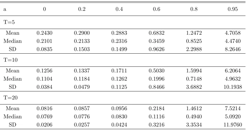
3.4 Experiments on Persistence
Now we consider the case when (Xit) is persistent. We generate zero-mean AR time series
as follows,
Xi,0 ∼N(0,2), and Xit=aXi,t−1+ηt,
where the a ∈ [0,1) controls the persistence level and ηt ∼ i.i.d. N(0,2(1−a2)). Hence
for each i, Xit is strictly stationary with marginal distribution N(0,2). αi is generated as
random effect, that is,αi∼ i.i.d.N(0,4) independent ofX. We use the plug-in bandwidth
described in Remark 4 following Theorem 2. We vary a from 0 to 0.95. The number of repetitions is set to be 500, and the mean, the median, and the SD (Standard Deviation)
of the ISE’s of FD estimator are reported in Table 2. We choose to report results from the
experiments onf2. The results from other functional forms are similar.
Table 2 shows, not surprisingly, that our estimator is unstable at high persistence levels.
Under mild persistence (a≤0.6), the mean, the median, and the SD of ISE still remain in a reasonable range. This is not the case whena≥0.8. Note that the median’s are generally lower than the mean, indicating there are instances where our estimator is way off the mark,
Table 1: Monte Carlo Results I: On Comparative Performance
This table compares the best performance of each estimator. The median and the SD of the smallest ISE of each estimator are reported. T = 5, the number of repetition is 500, and more details are in the text.
RE FE
σ= 0.5 σ= 1 σ= 0.5 σ= 1
Median SD Median SD Median SD Median SD
f1, N=50
FD 0.0232 0.0198 0.0668 0.0673 0.0160 0.0216 0.0656 0.1058
LL-RE 0.0424 0.0541 0.0713 0.0736 1.2478 0.5316 1.2001 0.6261
LL-LSDV 0.3668 0.0809 0.3932 0.1099 0.4641 0.1710 0.4934 0.2141
f1, N=100
FD 0.0123 0.0110 0.0364 0.0393 0.0089 0.0116 0.0311 0.0470
LL-RE 0.0262 0.0252 0.0389 0.0405 1.2059 0.3550 1.2287 0.3954
LL-LSDV 0.3618 0.0522 0.3813 0.0784 0.4386 0.1142 0.4478 0.1334
f2, N=50
FD 0.0964 0.0451 0.2501 0.1272 0.2566 0.2591 0.5421 0.4094
LL-RE 0.1658 0.0917 0.2602 0.1292 1.3758 0.5950 1.4073 0.6982
LL-LSDV 0.8486 0.1279 0.8781 0.1796 1.1034 0.2168 1.1536 0.2455
f2, N=100
FD 0.0515 0.0220 0.1436 0.0652 0.1868 0.1570 0.3506 0.2380
LL-RE 0.0981 0.0450 0.1458 0.0684 1.3030 0.4149 1.3522 0.4595
LL-LSDV 0.8296 0.0840 0.8394 0.1220 1.1009 0.1310 1.1197 0.1585
f3, N=50
FD 0.1358 0.0533 0.2991 0.1244 0.2722 0.1264 0.4955 0.1869
LL-RE 0.2126 0.0926 0.2972 0.1293 1.4589 0.5992 1.4709 0.6333
LL-LSDV 0.4988 0.0721 0.5323 0.0913 0.5313 0.0796 0.5630 0.0964
f3, N=100
FD 0.0731 0.0275 0.1832 0.0694 0.1974 0.0877 0.3921 0.1329
LL-RE 0.1262 0.0498 0.1875 0.0738 1.3840 0.4042 1.3636 0.4603
LL-LSDV 0.4965 0.0562 0.5134 0.0700 0.5247 0.0523 0.5530 0.0693
f4, N=50
FD 0.1371 0.0572 0.3153 0.1293 0.2852 0.1446 0.5131 0.2582
LL-RE 0.2142 0.0959 0.3167 0.1320 1.4372 0.6158 1.4939 0.6304
LL-LSDV 0.9792 0.1285 1.0267 0.1659 1.1119 0.1616 1.1327 0.1933
f4, N=100
FD 0.0776 0.0279 0.1879 0.0704 0.2022 0.1146 0.3897 0.1673
LL-RE 0.1288 0.0519 0.1867 0.0720 1.3883 0.4157 1.3787 0.4500
Table 2: Monte Carlo Results II: On Persistence
This table reports how persistence inXit may influence the performance of FD. Mean, Median, and SD of ISE are reported. ais the level of persistence. N= 50, the underlying function isf2, the number of
repetition is 500, and more details are in the text.
a 0 0.2 0.4 0.6 0.8 0.95
T=5
Mean 0.2430 0.2900 0.2883 0.6832 1.2472 4.7058
Median 0.2101 0.2133 0.2316 0.3459 0.8525 4.4740
SD 0.0835 0.1503 0.1499 0.9626 2.2988 8.2646
T=10
Mean 0.1256 0.1337 0.1711 0.5030 1.5994 6.2064
Median 0.1104 0.1184 0.1262 0.1996 0.7148 4.9632
SD 0.0384 0.0479 0.1125 0.8466 3.6882 10.1938
T=20
Mean 0.0816 0.0857 0.0956 0.2184 1.4612 7.5214
Median 0.0769 0.0776 0.0830 0.1116 0.4940 5.0920
SD 0.0206 0.0257 0.0424 0.3216 3.3534 11.9760
to caution against applying our estimator to panels of highly persistent time series.
To defend our methodology, we point out that the above data generating process is close
to the worst scenario of our estimator. Whena= 0.95, the conditional distribution ofXit
given Xi,t−1 =v is Gaussian with mean 0.95v and standard deviation 0.44. Let v= 0, for
example, the conditional densityp(u|v) is close to zero at{u:|u|>0.44·4 = 1.56}. Recall that we estimate functions on [−2,2] and that p(u|v) is implicitly on the denominator of the asymptotic variance.
4. Conclusions
In this paper we present a new methodology for estimating the nonlinear component of
semiparametric panel data models. Technically, we use first differencing transformation to
interest. We give the asymptotic properties of our estimator. And Monte Carlo simulations
show that our estimator performs reasonably well for finite samples.
References
Andrews, D. W. K., 1991, Asymptotic Optimality of Generalized CL, Cross-Validation,
and Generalized Cross-Validation in Regression with Heteroskedastic Errors, Journal
of Econometrics, 47, 359-377
Auestad, B., D. Tjøstheim (1991), Functional identification in nonlinear time series. In
G.G. Roussas (ed.), Nonparametric Functional Estimation and Related Topics
493-507, Amsterdam: Kluwer Academic.
Banerjee, A.V., and Duflo, E., 2003. Inequality and Growth: What Can the Data Say?,
Journal of Economic Growth, Springer, vol. 8(3), pages 267-99
Cleveland, W.S., 1979, Robust locally weighted regression and smoothing scatterplots,
Journal of the American Statistical Association, 74, 829-836.
Cai, Z., Masry, E., 2000, Nonparametric estimation in nonlinear ARX time series models:
Projection and linear fitting, Econometric Theory, 16, 465-501
Craven P., and G. Wabha, 1979, Smoothing noisy data with spline functions: Estimating
the correct degree of smoothing with generalized cross-validation, Numerische
Math-ematik, 31, 377-403.
Fan, J., 1992, Design-adaptive nonparametric regression, Journal of the American
Statis-tical Association, 87(420), 998-1004.
Fan, J. and Gijbels, I., 1992, Variable Bandwidth and Local Linear Regression Smoothers,
Fan, J., Hardle, W., Mammen, E., 1998, Direct Estimation of Low-Dimensional
Compo-nents in Additive Models, The Annals of Statistics, 26, 943-971
Gasser, T., A. Kneip, W. K¨ohler, 1991, A flexible and fast method for automatic
smooth-ing, Journal of the American Statistical Association, 86, 643-652
Gasser, T., H.-G. M¨uller, 1984, Estimating regression functions and their derivatives by
the kernel method, Scandinavian Journal of Statistics, 11, 171-185.
Henderson, D.J., R.J. Carroll, Q. Li, 2008, Nonparametric estimation and testing of fixed
effects panel data models, Journal of Econometrics, 144(1), 257-275.
H¨ardle, W., J.S. Marron, 1991, Bootstrap simultaneous error bars for nonparametric
re-gression, Annals of Statistics, 19(2), 778-796.
H¨ardle, W., E. Mammen 1993, Comparing nonparametric versus parametric regression
fits, Annals of Statistics, 21, 1926-1947.
Hengartner, N. W. and Sperlich, S., 2005, Rate optimal estimation with the integration
method in the presence of many covariates, Journal of Multivariate Analysis, 95,
246-272
Jones, M.C., S.J. Davies, B.U. Park, 1994, Versions of kernel-type regression estimators,
Journal of the American Statistical Association, 89(427), 825-832.
Kim, W., Linton, O.B., and Hengartner, N.W., 1999, A Computationally Efficient Oracle
Estimator for Additive Nonparametric Regression with Bootstrap Confidence
Inter-vals, Journal of Computational and Graphical Statistics, 8, 278-297.
Kneip, A., L. Simar, 1996, A general framework for frontier estimation with panel data,
Lee, Y., Mukherjee, D., 2008, New nonparametric estimation of the marginal effects in fixed
effects panel models: an application on the environmental Kuznets curve, Working
paper.
Li, K., 1987, Asymptotic Optimality for Cp, CL, Validation and Generalized
Cross-Validation, The Annals of Statistics, 15, 958-975
Li, Q., T. Stengos, 1996, Semiparametric estimation of partially linear panel data models,
Journal of Econometrics, 71(1-2), 389-397.
Linton, O.B., 1997, Efficient estimation of additive nonparametric regression models,
Biometrika, 84, 469-473
Linton, O.B., W. H¨ardle, 1996, Estimation of additive regression model with known links,
Biometrika, 83(3), 529-540.
Linton, O.B, Jacho-Chavez, D. 2009, On Internally Corrected and Symmetrized Kernel
Estimators for Nonparametric Regression, forthcoming in TEST, Springer.
Linton, O.B., J.P. Nielsen, 1995, A kernel method of estimating structured nonparametric
regression based on marginal integration, Biometrika, 82(1), 93-100.
Masry, E., Tjøstheim, D., 1997 Additive nonlinear ARX time series and projection
esti-mates, Econometric Theory, 13, 214C252
Mallows, C.L., 1973, Some Comments on Cp, Technometrics, 15, 661-675.
Mammen, E., Stove, B., and Tjostheim, D., 2009, Nonparametric additive models for
panels of time series, Econometric Theory, 25, 442-481.
Millimet, D.L., J.A. List, T. Stengos, 2003, The environmental Kuznets curve: real progress
Nadaraya, E.A., 1964, On estimating regression, Theory of Probability and its
Applica-tions, 9, 141-142.
Newey, W. K., 1994, Kernel Estimation of Partial Means and a General Variance
Estima-tor, Econometric Theory, 10, 233-253
Robinson, P.M., 1988, Root-N-consistent semiparametric regression, Econometrica, 56, 931-954.
Ruckstuhl, A. F., Welsh, A. H., Carroll, R. J., 2000, Nonparametric function estimation
of the relationship between two repeatedly measured variables, Statistica Sinica, 10,
51-71.
Ruppert, D., M.P. Wand, 1994, Multivariate locally weighted least squares regression,
Annals of Statistics, 22(3), 1346-1370.
Severance-Lossin, E. and Sperlich, S. (1999), Estimation of derivatives for additive
sepa-rable models, Statistics 33: 241-265.
Severini, T.A. and Staniswalis, J.G. 1994, Quasi-likelihood Estimation in Semiparametric
Models, Journal of the American Statistical Association, 89, 501-511
Stone, C.J., 1977, Consistent nonparametric regression (with discussion), Annals of
Statis-tics, 5, 595-645.
Su, L., Ullah, A., 2006, Profile likelihood estimation of partially linear panel data models
with fixed effects, Economics Letters, 92, 75-81
Su, L., Ullah, A., 2007, More efficient estimation of nonparametric panel data models with
random effects, Economics Letters, 96, 375-380.
Tjøstheim, D., Auestad, B.H., 1994, Nonparametric Identification of Nonlinear Time
Wand, M.P., M.C. Jones, 1993, Comparison of smoothing parameterizations in bivariate
kernel density estimation, Journal of the American Statistical Association, 88(422),
520-528.
Watson, G.S., 1964, Smooth regression analysis, Sankhy¯a, Series A, 26, 359-372.
Appendix I
Proof for Theorem 2: Theorem 1 establishes root-N consistency for ˆβ. In the following we may treat Rit= ∆Yit−∆Zit′ β as known. And we have
ˆ
f(u)−f(u) =
Z
[ ˆm(u, v)−m(u, v)]q(v)dv,
where the integration is taken on C ⊂Rd. Throughout the proof we suppress the domain for notational simplicity. Let Υ = [eit] and M = [m(Xit, Xi,t−1)]. By standard argument
in multivariate kernel regression asymptotics, and the assumptions that (i) (Xit, eit) is
i.i.d. across i, (ii) (Xit is stationary over t with T fixed, (iii) p2 is continuously partially
differentiable, (iv) f (hence m) is at least twice continuously partially differentiable, and other conditions on the kernel and the associated bandwidth matrix, we have
ˆ
m(u, v)−m(u, v) = ι′(Γ′WΓ)−1Γ′WΥ
+ι′
(Γ′WΓ)−1Γ′W(M−Γ
m(u, v) Dm(u, v)
)
+op(tr(H2)).
LetU1 andU2 denote the first and the second terms on the right, respectively. U2 gives us
the desired asymptotic bias, which is an integration of,
N2/(4+d)1
2µ2(k)tr
¡
(I2⊗H2)Hm(u, v)
¢
= N2/(4+d)1
2µ2(k)
£
tr¡H2Hf(u)
¢
−tr¡H2Hf(v)
¢¤
= 1 2µ2(k)
£
We now examine U1. Letn=N T. We first write
U1 =ι′
µ
1
nΓ
′WΓ
¶−1µ
1
nΓ
′WΥ
.
Use the fact thatXit is stationary andT is fixed, we use standard arguments to obtain
ι′
µ
1
nΓ
′WΓ
¶−1
=
µ
p2−1+op(1) −p2−2∂p2∂u′ +op(1) −p− 2
2 ∂p2∂v′ +op(1)
.
Note thatop(1) is uniform, for which we require N|H|2→ ∞, which means d <4. Hence
U1 = (A1(u, v) +A2(u, v) +A3(u, v))(1 +op(1)),
where
A1(u, v) = p−21(u, v)
1 n N X i=1 T X t=1
KH(Xit−u)KH(Xi,t−1−v)eit,
A2(u, v) = −
µ
∂p2
∂u′p− 2 2
(u, v)1
n N X i=1 T X t=1
KH(Xit−u)KH(Xi,t−1−v)(Xit−u)eit
A3(u, v) = −
µ
∂p2
∂v′p
−2
2
(u, v)1
n N X i=1 T X t=1
KH(Xit−u)KH(Xi,t−1−v)(Xi,t−1−v)eit.
In the following, we show that
N2/(4+d)
Z
A1(u, v)q(v)dv →dN(0, V(u)),
and thatN2/(4+d)RA2(u, v)q(v)dv and N2/(4+d)
R
A3(u, v)q(v)dv are negligible
We first examineN2/(4+d)R A1(u, v)q(v)dv,
N2/(4+d)
Z
A1(u, v)q(v)dv = N2/(4+d)1
n
X
i,t
eitKH(u−Xit)
Z K
H(v−Xi,t−1)
p2(u, v)
q(v)dv
= N2/(4+d)1 n
X
i,t
eitKH(u−Xit)
µ
q(Xi,t−1)
p2(u, Xi,t−1)
+op(tr(H))
= √1
N
X
i
ξi,N +op(1),
where ξi,N = N−d/(2(4+d))T−1PteitKH(u−Xit)q(Xi,t−1)p−21(u, Xi,t−1). Note that the
integration on the right is a convolution involving the function KH which reduces to a
generalized delta function in the limit.
(ξi,N) is a triangular array and it can be observed that for eachN, (ξi,N) are i.i.d. with
zero mean. Next we calculate the second moment. We write
E(ξi)2 =N−d/(4+d)W1+N−d/(4+d)W2,
where
W1 =
1
T2E
X
t
e2itKH2(u−Xit)q2(Xi,t−1)p−22(u, Xi,t−1)
W2 = 1
T2E
X
s6=t
eiteisKH(u−Xit)KH(u−Xis)q(Xi,t−1)q(Xi,s−1)p−21(u, Xi,t−1)p−21(u, Xi,s−1)
ForW1, we have
W1 =
1
T2
X
t
σ2t
Z 1
|H|2K(H− 1(u
−v))q2(y)p−2(u, y)p2(v, y)dvdy
= σ¯
2
T|H|
Z
K2(w)q2(y)p−2(u, y)p2(u+Hw, y)dwdy
= ¯σ
2ϕd(k)
T|H|
Z
q2(y)p−1(u, y)dy(1 +op(1)).
Ee1te1s and ¯γ =T−2Ps6=tγt,s. It is obvious that ¯γ <∞. We have for W2,
W2 = 1
T2
X
s6=t
γt,s
Z
KH(u−x)KH(u−r) q(y)q(v)
p2(u, y)p2(u, v)
p2,t,s(x, y, r, v)dxdydrdz
= ¯γ|H|−2
Z
K(H−1(u−x))K(H−1(u−r)) q(y)q(v)
p2(u, y)p2(u, v)
p2,t,s(x, y, r, v)dxdydrdz
= ¯γ
Z
K(w)K(z)q(y)q(v)p−21(u, y)p−21(u, v)p2,t,s(u+Hw, y, u+Hz, v)dwdydzdv
= ¯γ
Z
q(y)q(v)p2−1(u, y)p2−1(u, v)p2,t,s(u, y, u, v)dydv(1 +op(1))<∞
Hence
Eξ2i = N−d/(4+d)σ¯
2ϕd(k)
T|H|
Z
q2(y)p−1(u, y)dy(1 +op(1)) +Op(N−d/(4+d))
= σ¯
2ϕd(k)
T|H0|
Z
q2(y)p−1(u, y)dy+op(1).
To see the asymptotic order of N2/(4+d)RA2(u, v)q(v)dv, we only need to examine
N−d/(4+d)Ee2itKH2(Xit−u)p−24(u, Xi,t−1)
µ
∂p2
∂u′(u, Xi,t−1)(Xit−u)
¶2
q2(Xi,t−1)
= N−d/(4+d) σ
2 t
|H|2
Z
K2(H−1(v−u))p−24(u, y)
µ
∂p2
∂u′(u, y)HH− 1(v
−u)
¶2
q2(y)p2(v, y)dvdy
= N−d/(4+d) σ
2 t
|H|
Z
K2(w)p−24
µ
∂p2
∂u′(u, y)H0w
¶2
q2(y)p2(u+Hw, y)dwdy·N−2/(4+d)
= Op(N−2/(4+d)).
Hence N2/(4+d)R A2(u, v)q(v)dv is asymptotically negligible. Similarly we can check that
N2/(4+d)RA3(u, v)q(v)dv is also negligible asymptotically.
To apply the Liapounov’s CLT to √1 N
P
iξi,N, we need to check whether the following
holds for some constant ǫ >0,
N
X
i=1
E|ξi,N/
√
The above is equivalent to
N−ǫ/2E|ξ1,N|2+ǫ→0, asN → ∞.
Observe that| · |2+ǫ is a convex function, hence
|ξi,N|2+ǫ≤N−d(2+ǫ)/(2(4+d))
1
T
T
X
t=1
¯
¯eitKH(u−Xit)q(Xi,t−1)p−21(u, Xi,t−1)
¯ ¯2+ǫ
.
And by the positiveness ofk,q, and p2, and the independence ofeit from (Xit), we have
E¯¯eitKH(u−Xit)q(Xi,t−1)p−21(u, Xi,t−1)
¯ ¯2+ǫ
= E|eit|2+ǫE
¯
¯KH(u−Xit)q(Xi,t−1)p−21(u, Xi,t−1)
¯ ¯2+ǫ
= E|eit|2+ǫ|H|−(2+ǫ)
Z
K(2+ǫ)(H−1(u−x))q2+ǫ(y)p−2(2+ǫ)(u, y)p2(x, y)dxdy
= E|eit|2+ǫ|H|−(1+ǫ)
Z
K(2+ǫ)(w)q2+ǫ(y)p2−(2+ǫ)(u, y)p2(u+Hw, y)dwdy
= |H|−(1+ǫ)E|eit|2+ǫ
Z
K(2+ǫ)(w)dw
Z
q2+ǫ(y)p2−(1+ǫ)(u, y)dy(1 +op(1))
= O(N(1+ǫ)/(4+d)),
since bothkand q are bounded,p2 is bounded from zero, andE|eit|2+ǫ ≤¡E|eit|4+2ǫ¢1/2<
∞. Hence
N−ǫ/2E|ξ1,N|2+ǫ=O(N−(1+ǫ)(d−1)/(4+d)−2ǫ/(4+d)) =o(1).
Hence the condition in (25) is verified. Now we apply the Liapunov’s CLT to the triangular