Munich Personal RePEc Archive
Dynamic analysis of the business failure
process: A study of bankruptcy
trajectories
du Jardin, Philippe and Séverin, Eric
Edhec Business School
1 July 2010
Online at
https://mpra.ub.uni-muenchen.de/44379/
du Jardin, P., Séverin, E., 2010, Dynamic analysis of the business failure process: A study of bankruptcy trajectories, proceedings of the 6th Portuguese Finance Network Conference, Ponta Delgada, Azores, July 1–3.
Dynamic analysis of the business failure process:
A study of bankruptcy trajectories
Philippe du Jardin
Edhec Business School 393, promenade des Anglais
BP 3116
06202, Nice cedex 3, France Email : [email protected]
Eric Séverin
Université de Lille 1 104 avenue du Peuple Belge
59000 Lille
Email: [email protected]
Abstract – This study examines a method of analyzing the dynamics of financial failure. Using
a large amount of data and a Kohonen map, we show how to depict company trajectories of
behavior and movement to terminal failure. We also show how to analyze these trajectories to
describe and understand the dynamics of bankruptcy and how to use them as a diagnostic tool.
Keywords – company failure, financial failure dynamics, bankruptcy trajectories
JEL classification – G33, C45, C59
1. Introduction
Most financial failure prediction models are designed to predict a company’s ability to
cover its financial obligations. To assess this ability, models usually measure a distance between
the financial situation of a company and a critical standard situation. This particular way of
forecasting is commonly used by most scoring systems; a prediction relies on the estimation of a
value that measures a distance to bankruptcy (Altman, 1968; Deakin, 1972; Ohlson, 1980; Odom
and Sharda, 1990; Tam and Kiang, 1992; Wilson and Sharda, 1994; Laitinen and Laitinen,
2000; Pompe and Bilderbeek, 2005; Agarwal and Taffler, 2008; Sueyoshi and Goto, 2009).
Such models suit creditors who need to assess the risk of non-reimbursement of their loans.
In this situation, failure is considered a “discrete event” (Altman, 1984).
However, one may also consider failure a process (Taffler, 1983; Balcaen and Ooghe,
2006). Indeed, failure is most often the result of a series of cascading events rather than a
statistical models that would not simply be scoring models but models able to estimate the
behavior of a company over time. From this point of view and particularly from the
company’s point of view, one may expect that these models would even make it possible for
companies to take corrective action to prevent bankruptcy (Slatter, 1984). Forecasting the
occurrence of an event then becomes less crucial than anticipating the dynamics of a behavior
that could lead to failure.
Research has highlighted the “paths” companies take during the years leading up to their
collapse. Some has concentrated on causes and relationships between variables that may
explain failure, as well as on the means of measuring them (Larson and Clute, 1979;
Preisendörfer and Voss, 1990; Kalleberg and Liecht, 1991; Hall, 1992; Lussier, 1995;
Sullivan et al., 1998). These studies provide a framework for analyzing how companies may fail,
depending on endogenous or exogenous variables and for how these variables may interact.
Other research has described the relationships between symptoms, and variables used as
proxies to assess these symptoms, in order to provide a dynamic understanding of the entire
process of failure. Miller and Frieson (1977), Sutton (1987), Hambrick and D’Aveni (1988),
or Mellahi and Wilkinson (2004), for example, have suggested general interpretation
frameworks highlighting chronological relationships between variables.
Still other work has attempted to show the chronological sequence of events that may
occur before failure (Argenti, 1976; Laitinen, 1991; Van Wymeersch and Wolfs, 1996; Ooghe
and De Prijcker, 2008), and hence, to find behavior common to different groups of companies.
When one analyzes the statistical methods used in the research that has just been presented,
one sees that, if they are not qualitative, those used to shed light on symptoms or relationships
betweens variables are well known and well established (all sorts of regression techniques,
factor analysis, correlation tests or test for differences between means). On the contrary, there
is no specific method that could be used to describe and analyze the dynamics of financial
failure. It is for this reason that we study this issue—bankruptcy dynamics—from a statistical
point of view. The aim of this research, then, is to provide a general framework that makes it
possible to represent the trajectories or the “paths” companies may take over the course of
their existence.
The remainder of this paper is organized as follows. In Section 2, we present a literature
review that explains our research questions. In Section 3, we describe the samples and
methods used in our experiments. Finally, in Section 4, we present and discuss our results; in
2. Literature review
Argenti (1976) is the first to have pointed out that companies might take different “paths”
before going bankrupt. Indeed, he provided a typology of trajectories that divides corporate
collapse into three groups. The first is made up of small, very young companies, the second of
medium-size, young companies and the third of mature companies.
Within each trajectory, Argenti analyzed the different steps in the failure process. His
analysis relies on a very small sample and is confined to factors almost completely internal to
the firms; hence his list of trajectories is far from exhaustive, and he doesn’t explain how the
three groups were determined.
With factor analysis, Miller and Friesen (1977) later attempt to find archetypal
relationships among variables that best describe healthy and failing companies. They finally
find ten different archetypes, six of them describing successful firms, and four, unsuccessful
firms. Although these profiles do not take into account changes that may affect companies
over time, they have the merit of highlighting a few groups of firms which behave in the same
manner or have characteristics in common, that is, which are likely to share a common
dynamics. This finding suggests that clustering companies in groups is likely to be the first
step towards understanding the dynamics of their behavior.
Hambrick and D’Aveni (1988) build on Argenti’s (1976) and on Miller and Friesen’s
(1977) work to design a comprehensive study related to the dynamics of failure, called
“downward spiral”. Their study, based on logistic regression, attempts to analyze changes in
financial ratios over time and compares the differences between sound and unsound big firms.
They find that decline can be broken up into four phases. This research leads not to the
profiling of failing companies but to a portrayal of the main phases in the failure of large firms.
Following these studies, two types of research were then done. Authors such as
Serrano-Cinca (1996) or Neophytou and Mar-Molinaro (2004) have designed models that attempt to
analyze patterns among failed and non-failed firms that dichotomous models are unable to
assess. Serrano-Cinca (1996) has used a Kohonen map to assess the ability of this method
precisely to describe categories of failed and non-failed companies which can be used to
better understand bankruptcy and to analyze the financial profile of any company from a
diagnostic perspective. Neophytou and Mar-Molinaro (2004) have done similar research, but
with a multi-dimensional scaling method. At the same time, other research, which attempts to
has also been done in this field. Using linear regression and a sample of failed firms, for
example, Thornhill and Amit (2003) find that firm age accounts for these differences.
Other research, most often using ratio-based analysis, has concentrated on the failure
process itself to shed light on how companies behave over time. Beaver (1966) is the first to
have provided a statistical analysis of the dynamics of financial ratios, showing how these
ratios could vary over time in keeping with a probability of bankruptcy. Later, other authors
have attempted to study how ratios behave according to variables that may affect the financial
structure of companies. Van Wymeersch and Wolfs (1996), for example, study a sample of
Belgian companies over a five-year period. The firms did not always have the same ratios, but
they had persistent characteristics in common: bankrupt firms, as failure approached, showed
a constant decrease in profitability, increased funding through external creditors funds and
just before bankruptcy, a considerable decrease in cash flow and a steady growth in the
percentage of added value devoted to cover fixed costs. At the same time, all these variables
remained constant in successful companies. Other research dealing with the failure process
has attempted to explain this phenomenon. Ooghe and De Prijcker (2006), using twelve case
studies, find four “paths” using data that described the organization, the strategy and the
products of companies, which are quite similar to the three trajectories found by Argenti
(1989). D’Aveni (1989) uses a small sample of firms filing for bankruptcy and data measured
over a five-year period to study the existence and the measure of patterns of decline. Failed
firms were classified into patterns by cluster-analysis, and D’Aveni finds three patterns of
decline: lingering firms, gradually declining firms, and rapidly declining firms.
We can notice a clear distinction between the two types of research we have just described:
the first is an attempt to design archetypes of failing companies that can move differently to
terminal failure without taking into account the time dimension; the second is an attempt to
assess patterns of decline over time.
Only very few studies have attempted to reconcile these two approaches. Laitinen (1991)
analyzes failure processes using financial ratios, over a period of six years. To assess these
processes, he first uses principal component analysis to classify companies in groups. He then
analyzes the behavior of a set of financial ratios, within each group, over this six-year period.
He finally finds three different “paths” explaining three distinct ways for a company to go
bankrupt. By the same token, Kiviluoto (1998), using financial ratios and a Kohonen map, also
analyzes failure processes, over a three-year period, but in a different manner. First, he
designs three maps, one per annual account, and he calculates the position of each company on
maps from the three consecutive years. On this final map, each vector represents a trajectory.
Instead of analyzing all these trajectories to look, as Laitinen does, for a few “paths” reflecting
typical behavior, he looks for a few groups of failing companies with similar patterns of behavior.
Our research strives to complement this work by taking an approach similar to Laitinen’s,
but based on a Kohonen map rather than on principal component analysis. After all, a Kohonen
map is able to handle non-linear relationships between variables, which are more likely the
true relationships between financial variables and a probability of bankruptcy (Laitinen and
Laitinen, 2000). A map is therefore perfectly well suited to dealing with these issues.
Thus, our research is to assess how to use a Kohonen map to quantify typical bankruptcy
trajectories, to analyze how such quantification may contribute to the understanding of
bankruptcy and how it can be used to prevent a company from going bankrupt. It is inspired
by the work of Gaubert and Cottrell (1999).
3. Samples and methods
To study bankruptcy trajectories, we have settled on a quantitative approach based solely
on accounting data computed using balance sheets and income statements. We have focused
our research on small- and medium-size companies, because these companies are more likely
to go bankrupt than larger companies.
A trajectory is considered a variation of the financial health of a company, measured at
different points in time. So, like Laitinen (1991), we have collected data over a six-year
period, a timeframe long enough to observe significant changes in the financial situation of
firms. As a consequence, we have excluded from our sample young firms, for which it is
obviously impossible to analyze behavior.
3.1. Samples and variables
We have collected three different data sets. The first was used to select a set of variables.
These variables were then used, with a second sample, to estimate trajectories, and these
trajectories were then validated with a third sample. The samples were selected using a
French database, Diane, and consisted of companies in the retail sector; in France, this sector
traditionally accounts for the largest percentage of failed firms. Within this set of companies,
we selected firms with an asset structure as homogenous as possible to control for the size
effect and to allow comparisons of ratios (Gupta, 1969). We ran an Anova and a
Mann-Whitney test on several breakdowns to find the most homogenous group, as well as a group
assets of less than €750,000. Data were gathered within a period of eight years, from 1996 to
2003, a steady state period from an economic point of view. Data are exclusively accounting
data and we computed only financial ratios (and one variation over two years of a financial
statement).
The first sample was selected to ensure that variables will be able to correctly discriminate
between failed and non-failed companies, and, hence, to ensure that trajectories will properly
reflect the behavior of these two types of firm. For this first sample, we collected data within
a single year, 2002, and we included just one variable (shareholder funds) from the previous
year (2001). When we selected healthy companies, we chose only companies in very good
shape, that is, companies that were still in business in 2005. Moreover, we selected companies
in operation for at least four years, because during the very first years of their lives, young,
healthy companies often have a financial structure similar to that of failing companies. We
also took into account the history of companies so as to select healthy firms that did not fail in
the previous four years. Indeed, for several years after being reorganized, firms that went
bankrupt and were then reorganized may reflect this bankruptcy in their financial statements
and hence may closely resemble failing companies. Bankrupt companies were selected only if
they were liquidated or reorganized in 2003, and at least 16 months after the publication of
the annual report from 2002 so as to avoid any intentional distortion of financial statements.
We tried to design a well-balanced sample of young and old firms because young companies
usually have a much higher probability of bankruptcy than older ones. Finally, we selected
bankrupt companies for which accounting data were available in 2002, and shareholder funds
available in 2001, and for which bankruptcy was declared (liquidation or reorganization) by
court decision in 2003. This first sample is made up of 250 healthy and 250 bankrupt companies.
Unsound firms were selected from among 1,548 failed firms in the retail sector and stored in the
French database, Diane (in 2003, 10,136 firms in the retail sector went bankrupt in France,
according to Insee).
We selected a second sample, made up of companies from the same sector and with the
same amounts of assets, but data were from 1996 to 2002 in order to compute financial ratios
along six consecutive years (1997 to 2002, because one variable is a variation of a financial
statement over two consecutive years). Healthy companies were randomly selected from
among those that were active in 2003, and bankrupt companies were also randomly selected
from among companies that were liquidated or reorganized by court decision in 2003. This
second sample is made up of 740 healthy and 740 bankrupt companies. None of the
We selected a third sample, identical to the second one, but data were from 1997 to 2003.
Healthy and bankrupt companies were also randomly selected, but with a one-year lag on the
previous sample (sound companies were still active in 2004 and unsound companies were
declared bankrupt in 2004). This second sample is made up of 325 healthy and 325 bankrupt
companies. None of the companies included in this sample was included in the previous
samples.
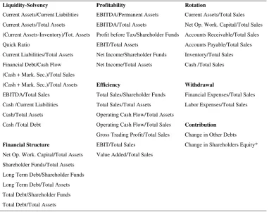
Finally, we chose a set a set of 41 initial variables (Table 1) that can be broken up into
seven somewhat arbitrary categories that best describe company financial profiles:
[image:9.595.73.456.283.584.2]liquidity-solvency, financial structure, profitability, efficiency, turnover, withdrawal and contribution.
Table 1: Initial set of variables
Liquidity-Solvency Profitability Rotation
Current Assets/Current Liabilities EBITDA/Permanent Assets Current Assets/Total Sales Current Assets/Total Assets EBITDA/Total Assets Net Op. Work. Capital/Total Sales (Current Assets-Inventory)/Tot. Assets Profit before Tax/Shareholder Funds Accounts Receivable/Total Sales Quick Ratio EBIT/Total Assets Accounts Payable/Total Sales Current Liabilities/Total Assets Net Income/Shareholder Funds Inventory/Total Sales Financial Debt/Cash Flow Net Income/Total Assets Cash /Total Sales (Cash + Mark. Sec.)/Total Sales
(Cash + Mark. Sec.)/Total Assets Efficiency Withdrawal
EBITDA/Total Sales Total Sales/Shareholder Funds Financial Expenses/Total Sales Cash /Current Liabilities Total Sales/Total Assets Labor Expenses/Total Sales Cash/Total Assets Operating Cash Flow/Total Assets
Cash /Total Debt Operating Cash Flow/Total Sales Contribution
Gross Trading Profit/Total Sales Change in Other Debts
Financial Structure EBIT/Total Sales Change in Shareholders Equity*
Net Op. Work. Capital/Total Assets Value Added/Total Sales Shareholder Funds/Total Assets
Long Term Debt/Shareholder Funds Long Term Debt/Total Assets Total Debt/Shareholder Funds Total Debt/Total Assets
* Change in Shareholders Equity was calculated without taking into account profit and loss Mark. Sec.= Marketable Securities – Net Op. Work. Capital: =Net Operating Working Capital
3.2. Variable selection methods
So as to select ratios which allow good discrimination between failed and non-failed firms, and
which are not sample- and selection-criteria-dependent, we have used several selection methods.
We first selected three parametric methods commonly used in the financial literature. We
variable combinations, a Fisher F test to interrupt the search, and a Wilks’s lambda to compare
variable subsets and determine the “best” one (Altman, 1968). We also selected two other
techniques: a forward stepwise search and a backward stepwise search, with a likelihood statistic
as an evaluation criterion of the solutions and a Chi2 as a stopping criterion (Ohlson, 1980).
However, these methods rely on the hypothesis that input-output variable dependence is
linear. As there is no evidence to think that this assumption is valid and that the relationship
between a probability of bankruptcy and independent variables is linear (Laitinen, 2000), we
chose three other non-parametric methods optimized for a non-linear context that are always
used in conjunction with neural networks; two of them evaluate the variables without using
the inductive algorithm (filter methods) and one uses the algorithm as an evaluation function
(wrapper method) (Leray and Gallinari, 1998). The first is a zero-order technique, which uses
the evaluation criteria designed by Yacoub and Bennani (1997), and the second is a first-order
method that uses the first derivatives of network parameters with respect to variables as an
evaluation criterion. The last one relies on the evaluation of an out-of-sample error calculated
with the neural network. To estimate this error, each sample used during the selection, the
process for which is presented below, was divided into two parts: 250 firms (125 healthy and
125 bankrupt) were used during the learning phase, and the other 250 firms were used to
compute the error. With all these criteria, we used only a backward search procedure, rather
than a forward or a sequential search, network parameters were determined a priori, and the
network was retrained after each variable removal.
To select variables, 1,000 random bootstrap samples were drawn with replacement from
the first sample (year 2002, 500 companies). Each bootstrap sample included 500 companies.
We used the following three-step procedure to select variables.
In the first step, each selection method was used to select variables with these 1,000
bootstrap samples. Then, to identify important variables, those that were included in more
than 70% of the selection results were selected. But this procedure might lead to the removal
of highly correlated variables. Indeed, if two variables are correlated, the selection results may
contain one or the other of these two variables, whereas none of them will be included in 70%
of the results. To avoid discarding potentially relevant but highly correlated variables, we
took a second step.
In the second step, variable pairs in which at least one variable was included in more than
90% of the bootstrap selections were considered pairs containing a relevant variable. Then, for
Finally, in the third step, variables that were selected in the first and second steps were used to
choose the final subsets. To choose these final subsets, the process used in the first step was
repeated once. We then compared the six final sets and chose the variables that were selected at
least twice.
3.3. Profile and trajectory design
A trajectory is a path along which a company moves from one class of risk to another over
time. These classes of risk can be considered the hierarchies of financial profiles that best
summarize all company financial situations. To design trajectories, we used a 10 x 10
Kohonen map, and data from the second samples (1,480 companies). A Kohonen map is
made up of a set of neurons (vectors) organized in two layers. The first, an input layer, is a
single neuron e= (e1, ..., en), where n is the number of variables. The second, a map, is a set of
neurons organized most often within a square, rectangular or hexagonal grid. Each neuron is a
weight vector w = (w1, ..., wn), where n is again the number of variables. The neuron of the input
layer is fully connected to the neurons of the map.
To set the value of the weight vectors, we used data from year 2002 (second sample), that
is, data computed one year before bankruptcy. During the learning phase, all data vectors are
compared to all weight vectors through a distance measure. For each input vector, once the
nearest neuron is found, its weights are adjusted so as to decrease the distance between the
input vector and this neuron. The weights of all neurons located in its neighborhood are then
adjusted as well, but the magnitude of the variation is proportional to the distance between
them on the map. During this phase, the neighborhood radius gradually shrinks, depending on a
function to be defined a priori. This procedure is repeated until the end of the learning phase.
The algorithm is as follows:
step 1: set the size of the map, using l lines *c columns, then randomly initialize the weights.
step 2: set the input neuron values e = (e1, ..., en) using data from one company.
step 3: compute the distance between vector (e1, ..., en) and the weight vector (wk1, ..., wkn) of
each neuron wk and select neuron wc with the minimum distance: ||e − wc|| = min{||e − wk||}
step 4: update weights within the neighborhood of wc:
wk(t +1) = wk(t)+(t)*hck(t)*(e(t) − wk(t))
where t is time, (t) the learning step, hck(t) the neighborhood function, and e(t) the input vector.
The neighborhood function is traditionally a decreasing function of both time and the distance
step 5: repeat step 2 to step 5 until t reaches its final value.
When the learning process is done, the resulting map is a nolinear projection of an
n-dimension input space onto a two-n-dimension space, which preserves the structure and
topology of input data relatively well (Cottrell and Rousset, 1997): two companies that are
close to each other in the input space will be close on the map. As the classes are known
(failures vs. survivors), each neuron can be labeled with the label of the class for which it
appears as a prototype (Rauber, 1999). To do so, all input vectors are once again compared to
all neurons. The percentage of companies belonging to each class that are the closest to each
neuron is then computed. Finally, the neurons are labeled with the label of the class whose
percentage is the highest.
When neurons are labeled, the map can be used to visualize the location of the neurons
belonging to each class. It gives a complete picture of proximities between failed and
non-failed firms on the map, and makes it possible to represent a “failure” and a “non-failure
space” and the boundaries between them. Once the map has been designed, trajectories were
computed. As we have collected data over six-year periods, each company can be represented
using six vectors, one for each year (1997 to 2002). To locate a position of a company on the
map, we have computed the distance between all neurons and the six vectors. Then, the
neurons which are the closest to each vector represent the different positions of a company on
the map over time. Each sequence of positions can be considered a trajectory. However, as the
map is made of 100 neurons, it becomes impossible to analyze and visualize all trajectories.
To reduce the number of combinations, we have attempted to group neurons into a few
meta-classes. Each class of neurons was analyzed separately so as to look for groups representing
solely healthy companies, and other groups representing solely non-healthy companies.
We conducted a hierarchical ascending classification, using three different aggregation
criteria (average linkage, complete linkage and Ward criterion), and we analyzed a few
partitions (Vesanto and Alhoniemi, 2000). Within each partition, all neurons were assigned to
a distinct meta-class, and were labeled. When two or three criteria led to a similar result, a
neuron was labeled with the class predicted using these two or three criteria. When the three
criteria led to different results, a neuron was labeled using a majority voting scheme,
depending on the class of its nearest neighbors. To select the best partition, we then compared
the different ones, in terms of homogeneity, using several indexes. We used the three best indexes
mentioned in the research done by Milligan (1981). Once the final partition was selected, the
To calculate trajectories, we classified the meta-classes according to an index of financial
health. Financial ratios were used to establish the hierarchy; once it was established, we
computed the different trajectories according to the initial position of each company on the
map, that is, the position in 1997. We first calculated company trajectories belonging to
meta-class 1, then company trajectories belonging to meta-meta-class 2, and so on. There are as many
sets of trajectories as meta-classes on the map. For each meta-class, we used a single-layer,
six-neuron Kohonen map to compute the trajectories. Six neurons were enough to quantify
correctly these data, because beyond six, some trajectories became indistinguishable from
others. Finally, we have analyzed these “paths to failure” and the differences that can be
observed between sound and unsound companies.
4. Results and discussion
4.1. Selected variables
Table 2 ranks the variables by frequency of appearance in the six sets of variables. Ten
[image:13.595.74.371.451.745.2]variables were selected at least twice; it was these variables we finally chose.
Table 2: Rank of the variables
Variables Number of
selections
Rank of appearance
in the six models
EBITDA/Total Assets 6 4 4 5 5 6 6 Shareholder Funds /Total Assets 5 1 1 2 3 7 Change in Shareholders Equity 5 1 3 3 4 7 (Cash + Mark. Sec.)/Total Assets 4 2 4 4 7 EBIT/Total Assets 3 2 4 5 Total Debt/Shareholder Funds 2 1 2
Cash/Total Debt 2 3 3 Cash /Current Liabilities 2 3 5
EBIT/Total Sales 2 5 6 Cash /Total Sales 2 7 8
Net Income/Total Assets 1 1 Cash/ Flow Total Assets 1 1 Current Assets/Current Liabilities 1 2 Profit before Tax/Shareholder Funds 1 2
(Cash + Mark. Sec.)/Total Sales 1 5 Operating Cash Flow/Total Sales 1 6
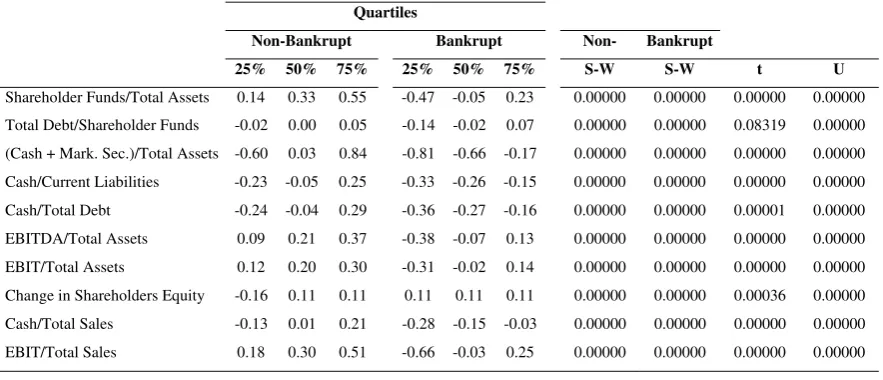
Table 3 shows the means and the quartiles of the distribution of these ten variables. The
figures describe the discrepancy of the deviations that exist within and between the two
groups of companies (figures computed using standardized data with zero mean and unit
variance). This table also shows the results of a Shapiro-Wilks normality test and the results
of two tests for differences between the means of each variable within each group. The
normality test indicates that none of the variables is normally distributed at the conventional
significance level of 5%. As a consequence, the non-parametric test (Mann-Whitney U test) is
more reliable than the parametric one (Student t test). This test shows that all variables present
[image:14.595.74.516.315.505.2]significant differences between the two groups.
Table 3: Characteristics of the selected variables
Quartiles – Normality test and tests for differences between the two groups
Quartiles
Non-Bankrupt Bankrupt Non- Bankrupt
25% 50% 75% 25% 50% 75% S-W S-W t U
Shareholder Funds/Total Assets 0.14 0.33 0.55 -0.47 -0.05 0.23 0.00000 0.00000 0.00000 0.00000 Total Debt/Shareholder Funds -0.02 0.00 0.05 -0.14 -0.02 0.07 0.00000 0.00000 0.08319 0.00000 (Cash + Mark. Sec.)/Total Assets -0.60 0.03 0.84 -0.81 -0.66 -0.17 0.00000 0.00000 0.00000 0.00000 Cash/Current Liabilities -0.23 -0.05 0.25 -0.33 -0.26 -0.15 0.00000 0.00000 0.00000 0.00000 Cash/Total Debt -0.24 -0.04 0.29 -0.36 -0.27 -0.16 0.00000 0.00000 0.00001 0.00000 EBITDA/Total Assets 0.09 0.21 0.37 -0.38 -0.07 0.13 0.00000 0.00000 0.00000 0.00000 EBIT/Total Assets 0.12 0.20 0.30 -0.31 -0.02 0.14 0.00000 0.00000 0.00000 0.00000 Change in Shareholders Equity -0.16 0.11 0.11 0.11 0.11 0.11 0.00000 0.00000 0.00036 0.00000 Cash/Total Sales -0.13 0.01 0.21 -0.28 -0.15 -0.03 0.00000 0.00000 0.00000 0.00000 EBIT/Total Sales 0.18 0.30 0.51 -0.66 -0.03 0.25 0.00000 0.00000 0.00000 0.00000 S-W: p-value of a Shapiro-Wilks normality test
t: p-value of a Student t test for differences between the means of the two groups
4.2. Classification with a Kohonen map: financial health segmentation
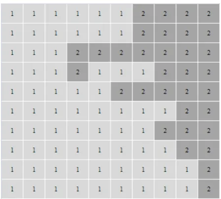
Figure 1 presents the Kohonen map and the distribution of non-bankrupt (1) and bankrupt
(2) companies within this “failure space”. We can notice on the map that the two groups were
quantified with two sets of relatively homogenous vectors, as there is no overlap. In addition,
each group is represented by a somewhat different number of neurons; healthy companies are
coded using 67 neurons, compared with 33 neurons for bankrupt companies. It seems that that
sound companies have a much wider variety of financial profiles than failing companies, with
some of them having profiles similar to those of failing companies. In the 200 papers dealing
with financial failure prediction that we analyzed and that have been published since the late
company will remain healthy in the near future than when they predict that it will fail, as if
the financial profiles of sound firms were much more complex and multiform than the profiles
of unsound ones. As a consequence, the profiles of some surviving companies seem to be
similar to the profiles of failing companies. Using a Kohonen map and financial ratios to
develop a typology of companies, Pérez (2003) noted that healthy firms would present a much
[image:15.595.70.295.233.435.2]wider spectrum of profiles than failing firms, without further analysis.
Figure 1: Kohonen map
1 Healthy companies – 2 Bankrupt companies
To design the meta-classes, we took into account the distribution of neurons by group of
companies. As the quantification of healthy firms requires twice as many neurons as the
quantification of the others, a “good” partition should highlight a wider variety of classes
representing the former than the latter.
Therefore, we have estimated the quality of the following partitions: 6-5, 6-4, 6-3, 6-2, 5-4,
5-3, 5-2, 4-3, 4-2; for example, 6-5 means that the partition is made of six meta-classes
encoding healthy companies, and five encoding failed ones.
Table 4 shows that partition 4-2 seems to be the best of those analyzed. This result is
consistent with the distribution of neurons within each class, since sound firms require twice
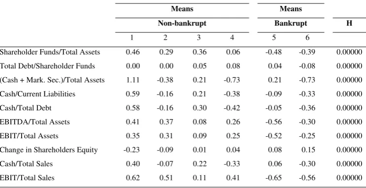
as many meta-classes as unsound ones. Table 5 reports the means of each variable within each
meta-class. These figures were computed using standardized data with zero mean and unit
Table 4: Rank of the partitions according to homogeneity indexes Number of meta- classes Point- Biserial Correlation C-Index - Hubert and Levin Gamma - Baker and Hubert Point- Biserial Correlation C-Index - Hubert and Levin Gamma - Baker and Hubert
Ranking Ranking Ranking 4-2 0.48042 0.12152 -0.17192 1 6 2
[image:16.595.77.449.332.523.2]5-2 0.47802 0.11632 -0.18399 2 4 3 4-3 0.46734 0.11630 -0.36749 3 3 4 5-3 0.46632 0.10943 -0.36847 4 1 5 5-4 0.43307 0.13105 -0.03695 5 8 1 6-2 0.42820 0.13274 -0.37586 6 9 6 6-4 0.41805 0.11673 -0.37685 7 5 9 6-3 0.41649 0.12328 -0.37685 8 7 8 6-5 0.41414 0.11448 -0.37635 9 2 7
Table 5: Characteristics of the variables within each meta-class
Means and test for differences between the six meta-classes
Means Means
Non-bankrupt Bankrupt H
1 2 3 4 5 6 Shareholder Funds/Total Assets 0.46 0.29 0.36 0.06 -0.48 -0.39 0.00000 Total Debt/Shareholder Funds 0.00 0.00 0.05 0.08 0.04 -0.08 0.00000 (Cash + Mark. Sec.)/Total Assets 1.11 -0.38 0.21 -0.73 0.21 -0.73 0.00000 Cash/Current Liabilities 0.59 -0.16 0.21 -0.38 -0.09 -0.33 0.00000 Cash/Total Debt 0.58 -0.16 0.30 -0.42 -0.05 -0.36 0.00000 EBITDA/Total Assets 0.41 0.37 0.08 0.26 -0.56 -0.30 0.00000 EBIT/Total Assets 0.35 0.31 0.09 0.25 -0.52 -0.25 0.00000 Change in Shareholders Equity -0.23 -0.09 0.01 0.04 0.08 0.15 0.00000 Cash/Total Sales 0.40 -0.07 0.22 -0.33 0.06 -0.30 0.00000 EBIT/Total Sales 0.62 0.51 0.11 0.41 -0.65 -0.56 0.00000 H: p-value of a Kruskal-Wallis test for the equality of the sum of ranks of each group
Table 6 synthesizes the financial characteristics of each meta-class using symbols such as
[image:16.595.74.330.640.759.2]“+” and “-”.
Table 6: General characteristics of the meta-classes
Non-bankrupt Bankrupt
The five dimensions depicted above are described by the following ratios: Financial structure: Shareholder Funds/Total Assets; Total Debt/Shareholder Funds
Solvency-Liquidity: (Cash + Mark. Sec.)/Total Assets; Cash/Current Liabilities; Cash/Total Debt Profitability: EBITDA/Total Assets; EBIT/Total Assets
Contribution: Change in Shareholders Equity Rotation: Cash/Total Sales
Efficiency: EBIT/Total Sales
Meta-class 1 is therefore made of companies in very good shape, with an outstanding
financial structure, very good liquidity and profitability, which are not relying on their
shareholders for fresh cash.
Meta-classes 2 and 3 are somewhat intermediary groups. They are made up of companies
that are rather healthy but have some differences: meta-class 2 is less liquid than meta-class 3,
but more profitable. And meta-class 4 is a category of companies which managed to survive
but which might have faced financial threats. Finally, meta-classes 5 and 6 are made up of
firms with the weakest situation; their financial structure is weak, meta-class 6 has the lowest
liquidity, whereas meta-class 5 is more liquid than meta-classes 2 and 4. These companies
may have attempted, by any means, to increase their income, and to shorten their payment
cycles, so as to escape the spiral of decline, but not sufficiently to avoid bankruptcy.
Meta-classes 5 and 6 are also made up of companies which relied heavily on their shareholders to
help them cope with their financial problems.
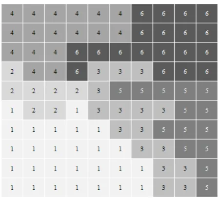
Figure 2 shows the six meta-classes within the Kohonen map. This map enables
visualization of proximities between groups better than that enabled by a list of figures; note
the distance between meta-classes 1 and 6, which are located on opposite sides of the map.
Also evident is the proximity between meta-classes 1 and 2, as well as the proximity between
parts of meta-classes 4 and 6, and parts of meta-classes 3 and 5. Meta-classes 3 and 4 are to
some extent the boundaries between typical healthy and bankrupt firms.
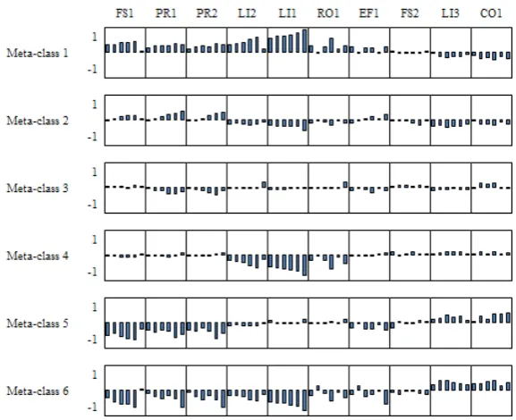
Figure 3 shows the distribution of financial ratios within neurons, using bar charts. This
figure makes it possible to visualize transitions between profiles in a single class and to assess
proximities between groups. Moreover, Figure 3 confirms the ordering of all groups defined
previously. Each graph is bounded by a horizontal line portraying the average of all ratios,
which is zero, as data are standardized. Firms located in the lower left part of the map have
ratios that are mostly above average, whereas those in the upper right part have ratios that are
Figure 2: Distribution of meta-classes on the map
Figure 3: Distribution of ratios within neurons
Each bar, for a given neuron, portrays one of the ratios listed in the following order: FS1 – FS 2 – LI1 – LI2 – LI3 – PR1 – PR2 – CO1 – RO1 – EF1
FS1: Shareholder Funds/Total Assets FS2: Total Debt/Shareholder Funds LI1: (Cash + Mark. Sec.)/Total Assets LI2: Cash/Current Liabilities LI3: Cash/Total Debt PR1: EBITDA/Total Assets PR2: EBIT/Total Assets
CO1: Change in Shareholders Equity RO1: Cash/Total Sales
4.3. Trajectory design
Based on this six-class hierarchy, we have considered class numbers ordered numerical
values that make possible a financial health or risk scale. These values were used to compute
trajectories. As stated above, a trajectory is the path a company takes through the space
depicted on the map under the action of financial forces, which is embodied by shifts from
one class of risk to another over time. The 1,480 trajectories we have computed were then
clustered by initial company position on the map, say 1997; using six Kohonen maps, one per
[image:19.595.71.290.276.452.2]meta-class, all trajectories were grouped into six sets. Figure 5 shows their distribution.
Figure 4: Distribution of trajectories by initial company position on the map
The six lines on Figure 4 display trajectories whose origin is meta-class 1, 2…, 6
respectively. On each graph, the scale of the X-axis corresponds to the six years, and the scale
of the Y-axis to the six meta-classes. The percentages in columns are the proportion of
companies belonging to each set of trajectories, and those in the lower part of each graph, the
same proportion but within each trajectory. The first line displays the behavior of companies
belonging to meta-class 1, that is, firms with the best financial health. The first four
trajectories show that most of these firms never shifted to the “bankruptcy space”, unlike the
last two trajectories, which show that, finally, some of them went bankrupt. The last line,
conversely, displays on the first two trajectories how companies in bad financial shape in
1997 have managed to improve, and on the last four trajectories how other companies, also in
bad shape, finally collapsed.
Figure 5 below shows the proportions of sound and unsound companies by trajectory. The
size of the white (grey) part of each graph, on Figure 5, is proportional to the number of
then complements Figure 5 in that it helps understand to what extent a given trajectory
describes behavior of survivors or behavior of failures.
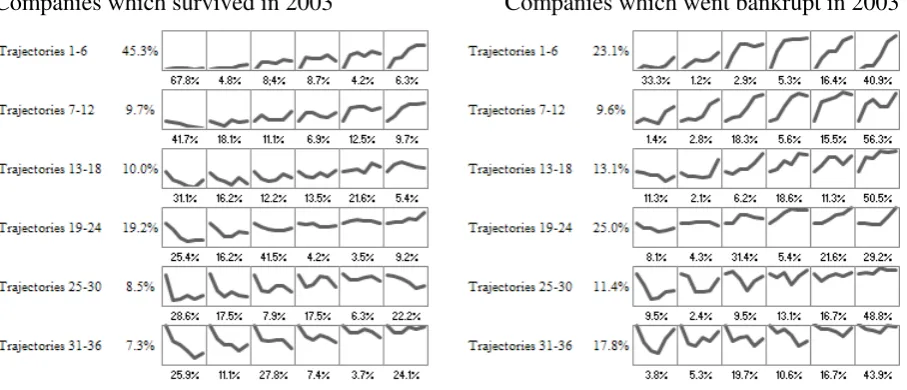
Figure 5: Proportions of sound and unsound companies in 2003 by trajectory
Figure 6 can be divided into two parts: the upper left half represents firms whose financial
profile was, on average, rather good in 2002, and most of which managed to survive in 2003.
Conversely, the lower right half corresponds to companies which faced financial troubles in
2002, and most of which went bankrupt in 2003.
4.4. Trajectory analysis
4.4.1. Company behaviors
Figure 6 exhibits the different behavior regarding the final status of companies. On the left,
it shows trajectories of healthy companies; on the right, trajectories of bankrupt companies.
Figure 6 suggests some interesting patterns. First, bankrupt firms have four major modes of
behavior in common. The first (trajectories 2 to 12) points to a sudden deterioration in the
health of firms four or five years before bankruptcy, without any further improvement. These
firms were initially healthy, but have almost certainly had to deal with a major event they were
unprepared for and defenseless against. The second (trajectories 14 to 18 and 21 to 24) reveals
slower but inexorable deterioration, with sometimes a period of (partial) remission. These are
mainly firms whose financial profiles, six years before bankruptcy, are rather average but
steadily weaken. The third mode (trajectories 25 to 28 and 31 to 34) is characterized by a period
of remission, in which companies shifted from a very difficult financial situation to a better
they were unable to adapt sufficiently to survive. The fourth mode (trajectories 29 and 30, 35
and 36) has to do with firms that were unsound for many years but never had the opportunity
[image:21.595.74.528.177.372.2]to get better even though they managed to survive for a long time.
Figure 6: Distribution of trajectories
Companies which survived in 2003 Companies which went bankrupt in 2003
Second, healthy companies share only three main forms of behavior. The first (trajectories
1 to 4, 7 to 9, 13 to 16) corresponds to firms whose financial situation, initially good, changed
little over time. Their trajectories are rather flat. The second (trajectories 19 and 20, 25 to 27,
31 to 33) consists of firms which experienced difficulty but were able to recover quickly. The
third (trajectories 11 and 12, 17 and 18, 23 and 24, 29 and 30, 35 and 36) corresponds to
companies which managed to survive despite a weak situation. Although this group is not that
large, because it is made of a small percentage of companies, it is considerably larger than the
group of companies that went bankrupt while they were in relatively good health.
Third, when one looks carefully at the shape of trajectories, one may notice that the
behavior of failed firms is much more chaotic than that of the others, as if these companies
were constantly seeking an equilibrium they were unable to achieve. Actually, sound firms
have a much wider variety of financial profiles than failing companies, as depicted by Figure
1, since accurate quantification requires many more neurons to encode the former than the
latter. However, their trajectories are less likely to exhibit the same variety. As a matter of
fact, failed firms exhibit wider movements of oscillation between meta-classes than the
others. It is for this reason that their trajectories are less compact. As it happens, we have
Regardless of the number of neurons, the map needs twice as many neurons to encode
trajectories of failed firms as to encode trajectories of healthy ones.
To deepen this statement, we have analyzed how the 1,480 firms of our sample behave
over time and shifted from one meta-class to another. For this purpose, we have computed, for
each company, the number of steps that occurred in the “healthy” part of the map, depicted by
Figure 2. We have counted the number of firms whose trajectory has oscillated only within
this “healthy part” (between meta-classes 1 and 4), without reaching the “non-healthy part”
(meta-classes 5 and 6). We then counted the number of firms with five steps within the
“healthy part”, then four steps, and so on, until those whose trajectory has oscillated only
[image:22.595.73.417.338.506.2]between meta-classes 5 and 6. Table 7 shows the results.
Table 7: Distribution of firm oscillations between “healthy” and “non-healthy” parts of the
Kohonen map
Companies declared healthy in 2003 Companies declared bankrupt in 2003
Number of steps within the “healthy
part” of the map
Number of companies
% Number of steps within the “non-healthy
part” of the map
Number of companies
%
6 431 58,2% 6 82 11.1% 5 138 18,6% 5 128 17.3% 4 75 10,1% 4 160 21.6% 3 51 6,9% 3 123 16.6% 2 20 2,7% 2 123 16.6% 1 17 2,3% 1 74 10.0% 0 8 1,1% 0 50 6.8%
Table 7 confirms (not unsurprisingly) that the trajectories of sound firms are less erratic
than those of unsound firms. A large proportion of successful firms always remain in the same
place, whereas failed firms tend to zigzag.
4.4.2. Evolution of financial ratios over time by meta-classes
Laitinen (1991) has demonstrated that the ability of financial ratios to discriminate between
failures and survivors depends on the distribution of failure processes among bankrupt companies.
Figure 7 clearly shows the discrepancies in the distributions of financial ratios between
meta-class1 and meta-classes 5 and 7. It also points out that the values of liquidity ratios LI1 and
L12 (Cash + Mark. Sec.)/Total Assets, Cash/Current Liabilities) are far below the average in
meta-classes 2, 4 and 6, and that those of profitability ratios PR1 and PR2 (EBITDA/Total
in other meta-classes. As a consequence, their ability to discriminate between meta-class 1
and meta-classes 5 and 6 is certainly greater than their ability to discriminate between others.
Figure 7 also indicates an interesting feature. Pompe and Bilderbeek (2005) hypothesize
that there should be a chronological order of decrease in values from different categories of
ratios during the successive phases before bankruptcy. They assume that when a firm is
heading towards bankruptcy a downward movement would first be seen in the values of the
profitability ratios, followed by the values of the solvency ratios, and finally the liquidity
ratios. But this hypothesis was not supported by their results. When one looks at Figure 7
from Pompe and Bilderbeek’s point of view, one sees that, as the risk of default increases,
firms are likely to face liquidity problems before they face other financial threats. Indeed,
liquidity ratios L1 and L2 within meta-classes 2 and 4 are much more affected by a downward
trend than other ratios. Profitability problems occur later; ratios PR1 and PR2 slowly slide
under the average within meta-class 3, but deteriorate dramatically within meta-classes 5 and
6. Thus, the way categories of financial ratios may behave over time, within a chronological
sequence, appears to be related more closely to the class of risk a company belongs to than to
the period before failure. A similar analysis, done using trajectories, closely mirrored the
order we mentioned above. Figure 8 exhibits the distribution of ratios between 1997 and 2002
of successful firms which moved along trajectories 1 to 6. And Figure 9 exhibits the same
[image:23.595.69.358.506.741.2]data but of failed firms which moved along trajectories 31 to 36.
Figure 7: Distribution of ratios by meta-class between 1997 and 2002
Figure 8: Distribution of ratios of successful firms by trajectories 1 to 6 between 1997 and 2002
Figure 9: Distribution of ratios of failed firms by trajectories 31 to 36 between 1997 and 2002
Figure 8 indicates that the order of decrease of ratios depends on the order of trajectories,
and that liquidity ratios have the greatest magnitude of decrease, which is slightly less for
those of profitability and even less for those of financial structure. This hierarchy is a bit more
difficult to observe on Figure 9. However, liquidity ratios appear to collapse first, before
profitability ratios. It is likely that a major reason for the failure of small- and medium-size
in shareholders equity changes as the risk of failure increases. Indeed, when these firms lack
liquidity and are unable to borrow, they are more likely to seek a cash injection from their
shareholders as their financial situation worsens.
4.4.3. Trajectories as a diagnostic tool
We have used our last sample of 650 companies to validate the 36 trajectories and check
their stability over time. This validation is a necessary condition to use them as a diagnostic
tool with a new sample. Data from this sample were projected onto the initial map to compute
trajectories. To estimate the distribution, a distance calculation was then used to compare the
650 trajectories and the 36 prototypes. Figure 10 exhibits the distribution of firms within each
category, and Table 8 reports the p-values of a test for differences between proportions to
[image:25.595.71.301.362.541.2]assess discrepancies.
Figure 10: Proportions of sound and unsound companies in 2004 by trajectory
Table 8: Test for differences between the percentage of firms belonging to sample 2002 and
firms belonging to sample 2003 within each meta-class and each trajectory
Meta-classes Trajectories
p-value p-value
[image:25.595.75.397.608.723.2]The distribution appears to be consistent to that of the sample used to design trajectories.
All p-values indicate that the distribution of firms among meta-classes is similar at the
conventional significance level of 5%, and that the same distribution among trajectories is
also similar in all cases but four (trajectories 15, 16 and 31) at the level of 5%. We have checked
only these differences using a sample drawn with a one-year lag on our initial sample.
Now, to illustrate how to study the profile and the behavior of a company, we have selected
three firms from the third sample, gathered data and computed financial ratios over a six-year
period: 1998 to 2003. We then calculated their trajectories. Figure 11 shows their behavior.
It is also possible to compute trajectories within a shorter period, four or five years, for
example. In such a case, the distance between a given trajectory and the 36 paths will be
computed while considering one or two missing values. One may then compute the two or three
[image:26.595.71.295.356.560.2]closest paths to that of a given company, to build different scenarios and broaden the analysis.
Figure 11: Three individual trajectories
Each set of lines, depicted with a different color, shows the behavior of a company. The steps are numbered and each one encodes a position on the map within a year: 1 is the position in 1998, 2 in 1999, 3 in 2000, 4 in 2001, 5 in 2002 and 6 in 2003.
The first trajectory (black lines) exhibits the behavior of a company that stayed healthy for
six years and is still in operation in 2010. The second one (gray lines) shows how a company
moved slowly along a path to failure; in 1998, its situation was fairly good, but as time went
by, its financial ratios progressively worsen and, finally, it went bankrupt in 2004. The third
one (white lines) exhibits a rather erratic trajectory. This firm was in bad shape in 1998, and
managed to recover two years later, but this remission was short. From 2001 to 2002 its
situation worsened, only to get better in 2003. The firm finally went bankrupt in 2005.
1
2 3
4 5
6
1
3 2
4 5
6
1
2 3
4 5
These examples indicate how to use the map to assess the class of risk a company belongs to,
and within this class of risk, to estimate to what extent its behavior may or may not lead to failure.
The method we have suggested here has the advantage of assessing a trend that, unlike
scoring methods, can provide only an index of health very often depending solely on
single-year data, takes into account the history of firms. It is now acknowledged that a significant
number of companies may show signs of financial weakness many years before failing
(Hambrick and D’Aveni, 1988). This information may then be used by a model based on
trajectories. It also has the advantage of highlighting risk factors by showing the variables or
ratios that exhibit weak values, hence weaknesses that require corrective action.
5. Conclusion
This research has shown how the dynamics of failure, conceptualized by some authors,
could be depicted using a statistical method usually applied to other issues. It has also shown
it makes it possible to discover specific behavior of firms and revelatory patterns of failure
not discovered by most data analysis methods.
The limitations of our study may serve to provide guidelines for future studies of failure.
One need is to explain the trajectories, using variables that were not included in our analysis,
and particularly qualitative variables; does firm age, for example, often studied as a cause of
failure, play a role? Levinthal (1991) has stated that age and experience could enhance a firm’s
survival value by providing a kind of cushion against failure. This factor might account for
some of the many trajectories we have highlighted. It is also possible that exogenous factors
play a significant role. It would also be worth taking a large number of variables to determine
if the order in which liquidity and profitability problems crop up depends on company
behavior. Finally, such trajectories could be analyzed within shorter intervals of time, three or
six months, for example. Indeed, corrective action taken by firms to stay in shape or to avoid
bankruptcy is hardly observable if data are collected in excessively large intervals.
References
Agarwal V., Taffler R. (2008), Comparing the Performance of Market-based and
Accounting-based Bankruptcy Prediction Models, Journal of Banking and Finance, vol. 32, pp. 1541-1551.
Altman E. I. (1968), Financial Ratios, Discriminant Analysis and the Prediction of Corporate
Altman E. I. (1984), The Success of Business Failure Prediction Models – An International
Survey, Journal of Finance, vol. 23, pp. 589-609.
Argenti J. (1976), Corporate Collapse: the Causes and Symptoms, New York, Wiley, Halsted
Press.
Balcaen S., Ooghe H. (2006), 35 Years of Studies on Business Failure: An Overview of the
Classical Statistical Methodologies and their Related Problems, British Accounting
Review, vol. 38, pp. 63-93.
Beaver W. H. (1966), Financial Ratios as Predictors of Failure, Empirical Research in Accounting,
Selected Studies, Journal of Accounting Research, Supplement, vol. 4, pp. 71-111.
Cottrell M., Rousset P. (1997), The Kohonen Algorithm: A Powerful Tool for Analysing and
Representing Multidimensional Quantitative and Qualitative Data, in J. Mira, R.
Moreno-Diaz, J. Cabestany, Lecture Notes in Computer Science, n° 1240, Springer, pp. 861-871.
D’Aveni R. A. (1989), The Aftermath of Organizational Decline: a Longitudinal Study of the
Strategic and Managerial Characteristics of Declining Firms, Academy of Management
Journal, vol. 32, pp. 577-605.
Deakin E. B. (1972), A Discriminant Analysis of Predictors of Business Failures, Journal of
Accounting Research, vol. 10, pp. 167-179.
Gaubert P., Cottrell M. (1999), A Dynamic Analysis of Segmented Labor Market, Fuzzy
Economic Review, vol. 4, pp. 63-82.
Gupta M. C. (1969), The Effect of Size, Growth, and Industry on The Financial Structure of
Manufacturing Companies, Journal of Finance, vol. 24, pp. 517-529.
Hall, G. (1992), Reasons for Insolvency amongst Small Firms – A Review and Fresh
Evidence, Small Business Economics, vol. 4, pp. 237-250.
Hambrick D. C., D’Aveni R. A. (1988), Large Corporate Failures as Downward Spirals,
Administrative Science Quarterly, vol. 33, pp. 1-23.
Kalleberg, A. L., Liecht K. T (1991), Gender and Organizational Performance: Determinants
of Small Business Survival and Success, Academy of Management, vol. 34, pp. 136-161.
Kiviluoto K. (1998), Predicting Bankruptcies with the Self-Organizing Map, Neurocomputing,
vol. 21, pp. 191-220.
Laitinen E. K. (1991), Financial Ratios and Different Failure Processes, Journal of Business
Finance and Accounting, vol. 18, pp. 649-673.
Laitinen E. K., Laitinen T. (2000), Bankruptcy Prediction: Application of the Taylor's Expansion
Larson C. M., Clute R. C. (1979), The Failure Syndrome, American Journal of Small
Business, vol. 4, pp. 25-43.
Leray P., Gallinari P. (1998), Feature Selection with Neural Networks, Behaviormetrika, vol.
26, pp. 145-166.
Levinthal D. A. (1991), Random Walks and Organizational Mortality, Administrative Science
Quarterly, vol. 36, pp. 397-420.
Luoma M., Laitinen E. K. (1991), Survival Analysis as a Tool for Company Failure
Prediction, Omega International Journal of Management Science, vol. 19, pp. 673-678.
Lussier, R. N. (1995), A Nonfinancial Business Success Versus Failure Prediction Model for
Young Firms, Journal of Small Business Management, vol. 33, n° 1, pp. 8-20.
Mellahi K., Wilkinson A. (2004), Organizational Failure: A Critique of Recent Research and
a Proposed Integrative Framework, International Journal of Management Review, vol. 5-6,
pp. 21-41.
Miller D., Friesen P. H. (1977), Strategy-Making in Context: Ten Empirical Archetypes,
Journal of Management Studies, vol. 14, pp. 253-280.
Milligan, G. W. (1981), A Monte Carlo Study of Thirty Internal Criterion Measures for
Cluster Analysis, Psychometrika, vol. 46, pp. 187-199.
Neophytou E., Mar-Molinero C., (2004), Predicting Corporate Failure in the UK: A
Multi-dimensional Scaling Approach, Journal of Business Finance and Accounting, vol. 31, pp.
677-710.
Odom M. C., Sharda R. (1990), A Neural Network Model for Bankruptcy Prediction,
Proceedings of the IEEE International Joint Conference on Neural Networks, San Diego,
California, vol. 2, pp. 163-168.
Ohlson J. A. (1980), Financial Ratios and the Probabilistic Prediction of Bankruptcy, Journal
of Accounting Research, vol. 18, pp. 109-131.
Ooghe H., De Prijcker S. (2008), Failure Processes and Causes of Company Bankruptcy: A
Typology, Management Decision, vol. 46, pp. 223-242.
Pérez, M. (2002), De l’analyse de la performance à la prévision de défaillance: les apports de
la classification neuronale, PhD Dissertation, Jean-Moulin University, Lyon III.
Pompe P. P. M., Bilderbeek J. (2005), The Prediction of Bankruptcy of Small- and
Medium-Sized Industrial Firms, Journal of Business Venturing, vol. 20, pp. 847-868.
Preisendörfer P., Voss T. (1990), Organization Studies, Organizational Mortality of Small
Rauber A. (1999), LabelSOM: On the Labeling of Self-Organizing Maps, in Proceedings of the
International Joint Conference on Neural Networks - IJCNN'99, Washington, DC, July 10-16.
Serrano-Cinca C. (1996), Self-Organizing Neural Networks for Financial Diagnosis, Decision
Support Systems, vol. 17, pp. 227-238.
Slatter S. (1984), Corporate Recovery, Successful Turnaround Strategies and Their Implementation,
Penguin Books, London.
Sueyoshi T., Goto M. (2009), Methodological Comparison between DEA (Data Envelopment
Analysis) and DEA-DA (Discriminant Analysis) from the Perspective of Bankruptcy
Assessment, European Journal of Operational Research, vol. 199, pp. 561-575.
Sullivan T. A., Warren E., Westbrook J. (1998), Financial Difficulties of Small Businesses
and Reasons for their Failure, U.S. Small Business Administration, Working Paper, n°
SBA-95-0403.
Sutton R.I. (1987), The Process of Organizational Death: Disbanding and Reconnecting,
Administrative Science Quarterly, vol.32, pp. 542-569.
Taffler R. J. (1983), The Assessment of Company Solvency and Performance Using a
Statistical Model, Accounting and Business Research, vol. 13, pp. 295-307.
Tam K. Y., Kiang M. Y. (1992), Managerial Applications of Neural Networks: The Case of
Bank Failure Predictions, Management Science, vol. 38, pp. 926-947.
Thornhill S., Amit, R. (2003), Learning about Failure: Bankruptcy, Firm Age, and the
Resource-Based View, Organization Science, vol. 14, pp. 497-509.
Van Wymeersch C., Wolfs A. (1996), La trajectoire de faillite des entreprises : une analyse
chronologique sur base des comptes annuels, Facultés Universitaires Notre-Dame de la
Paix, Département de Gestion de l'Entreprise, Namur, Working Paper, n° 218.
Vesanto J., Alhoniemi E. (2000), Clustering of the Self-Organizing Map, IEEE Transactions
on Neural Networks, vol. 11, pp. 586-600.
Wilson R. L., Sharda R. (1994), Bankruptcy Prediction Using Neural Networks, Decision
Support System, vol. 11, pp. 545-557.
Yacoub M., Bennani Y. (1997), HVS: A Heuristic for Variable Selection in Multilayer
Artificial Neural Network Classifier, Proceedings of the International Conference on