Slow running of the gradient flow coupling from 200??MeV to 4??GeV inNf=3QCD

Slow running of the gradient flow coupling from 200 MeV

to 4 GeV in

N

= 3 QCD

Mattia Dalla Brida,1 Patrick Fritzsch,2 Tomasz Korzec,3 Alberto Ramos,4 Stefan Sint,5 and Rainer Sommer1,6 1_{John von Neumann Institute for Computing (NIC), DESY, Platanenallee 6, 15738 Zeuthen, Germany}

2

Instituto de Física Teórica UAM/CSIC, Universidad Autónoma de Madrid, C/Nicolás Cabrera 13-15, Cantoblanco, Madrid 28049, Spain 3

Department of Physics, Bergische Universität Wuppertal, Gaußstr. 20, 42119 Wuppertal, Germany 4_{Theoretical Physics Department, CERN, CH 1211 Geneva 23, Switzerland}

5

School of Mathematics, Trinity College Dublin, Dublin 2, Ireland

6_{Institut für Physik, Humboldt-Universität zu Berlin, Newtonstr. 15, 12489 Berlin, Germany} (Received 17 November 2016; published 25 January 2017)

Using a finite volume gradient flow renormalization scheme with Schrödinger Functional boundary conditions, we compute the nonperturbative running coupling in the range2.2≲g¯2_GFðLÞ≲13. Careful continuum extrapolations turn out to be crucial to reach our high accuracy. The running of the coupling is always between one loop and two loop and very close to one loop in the region of 200MeV≲μ¼ 1=L_≲4GeV. While there is no convincing contact to two-loop running, we match nonperturbatively to the Schrödinger functional coupling with background field. In this case, we know theμ-dependence up to ∼100GeV and can thus connect to theΛ-parameter.

DOI:10.1103/PhysRevD.95.014507

I. INTRODUCTION

The energy dependence of the strong coupling constant αsðμÞin a physical scheme provides information on how

to connect the low and high energy regimes of QCD. Relating these very different domains of the strong interactions is key to providing a solid determination of the fundamental parameters of the Standard Model [1]. Lattice QCD is in principle an ideal tool for such studies. Observables defined at short Euclidean distances can be used for a nonperturbative physical coupling definition (see for example Ref.[2]and references cited therein), and its value can be extracted accurately via Monte Carlo simulations. A direct implementation of this program has to face the so-called window problem: the short Euclidean distance used to define the renormalization scale has to be both large compared to the lattice spacing a and small compared to the total size of the box (denoted byL) used in the simulation. Since the box has to be large enough to describe hadronic physics, computational constraints severely limit the range of renormalization scales that one can study.

Finite size scalingprovides an elegant solution for this problem [3]. Relating the renormalization scale μ with the finite size of the box viaμ¼1=L, the couplingg¯2ðLÞ

depends on only one scale.1 Lattices of different volumes can be matched, allowing us to compute thestep scaling function σðuÞ [3]. It measures how much the coupling changes when the renormalization scale changes by a fixed factor, which we set to 2,

σðuÞ ¼g¯2_ð2LÞj ¯

g2_ðLÞ¼u: ð1:1Þ

It can be considered a discrete version of the renormaliza-tion groupβ-function. The exact relation is

logð2Þ ¼−

Z ffiffiffiffiffiffiffip_σðuÞ ffiffi

u

p

dx

βðxÞ; ð1:2Þ

with the convention

βðg¯Þ ¼−L∂g¯ðLÞ

∂L g¯∼→0−b0g¯ 3_−b

1g¯5þ…; ð1:3Þ

where the universal coefficients in the asymptotic expan-sion take the values b₀¼9=ð16π2Þ and b₁¼1=ð4π4Þ in N_f ¼3 QCD.

Once σðuÞis known, one can choose a reference scale Lref and setu0¼g¯2ðLrefÞ. The recursive relation

u_k¼σ−1_ðu

k−1Þ; k¼1;…; ns ð1:4Þ

allows one to relate nonperturbatively the scale1=Lrefwith the scales2k=L_ref fork¼0;…; n_s. A few iterations suffice

Published by the American Physical Society under the terms of the Creative Commons Attribution 4.0 International license. Further distribution of this work must maintain attribution to the author(s) and the published article’s title, journal citation, and DOI.

to connect a hadronic low energy scale with the electro-weak scale.

This is the strategy of the ALPHA Collaboration. Using the so-called Schrödinger Functional (SF) scheme

[4,5], QCD with N_f¼0, 2 and N_f¼4quark flavors has been studied[6–8]. Of immediate relevance to the present work is the recent application of this technique to the high energy domain of N_f¼3 QCD [1]. There, the energy dependence of the strong coupling was studied between the electroweak scale and a reference scale 1=Lref ¼1=L0∼4GeV, defined by g¯2SFðL0Þ ¼2.012, with very high accuracy.

This strategy is theoretically very appealing but meets some difficulties if the reference scale 1=Lref is lowered further into the hadronic regime. The computational cost of measuring the SF coupling grows fast at low energies and in particular toward the continuum limit. Thus, it is challenging to reach the low energy domain characteristic of hadronic physics, especially if one aims at maintaining the high precision achieved in Ref. [1]. The recently proposed coupling definitions based on the gradient flow (GF) [9]are much better suited for this task. The relative precision of the GF coupling in a Monte Carlo simulation is typically high and shows a weak dependence on both the energy scale and the cutoff (see Ref.[10]for a recent review and more quantitative statements). Moreover, GF couplings can easily be used in combination with finite size scaling and a particular choice of boundary con-ditions [11–14].

In this work, we use the GF coupling defined with SF boundary conditions [12][denoted byg¯2_GFðLÞ] to connect nonperturbatively the intermediate energy scale 1=L₀ with a hadronic reference scale 1=L_had defined by the condition

¯ g2

GFðLhadÞ ¼11.31: ð1:5Þ

The main result of this paper is the relation

L_had¼21.86ð42ÞL₀: ð1:6Þ

As the reader will see, our choices of lattice discretization and scale1=Lhadare such thatLhadcan be related with the pion and kaon decay constants by using the CLS ensembles

[15]. This work therefore represents an essential step in the ALPHA Collaboration effort of a first principles determi-nation of the strong coupling constant and quark masses at the electroweak scale in terms of low energy hadronic observables [16,17].

The paper is organized as follows. In Sec.II, we fix our notation and introduce the details of our coupling defi-nition. Sec. III discusses general aspects of taking the continuum limit, while Sec.IV contains the extraction of the continuum σðuÞ. After arriving at our main result in Sec. V, we discuss our findings in Sec. VI.

II. RUNNING COUPLING

A. Continuum

We work in four-dimensional Euclidean space and consider standard SF boundary conditions with zero back-ground field[4,5]. In summary, gauge fields are periodic in the three spatial directions with periodL, and the spatial components k¼1, 2, 3 of the gauge field satisfy homo-geneous Dirichlet boundary conditions in time,

Akð0;xÞ ¼AkðT;xÞ ¼0: ð2:1Þ

Fermion fields are required to obey periodic boundary conditions in space up to a phase,

ψðxþLkˆÞ ¼e{θ_ψðxÞ; ¯

ψðxþLkˆÞ ¼e−{θ_{ψ¯ðxÞ: ð2:2Þ}

We choose the valueθ¼1=2[18]. Defining the projectors P¼1₂ð1γ0Þ, the time boundary conditions read

Pþψð0;xÞ ¼0¼ψ¯ð0;xÞP−;

P₋ψðT;_xÞ ¼0¼ψ¯ðT;_xÞP_þ: ð2:3Þ

The GF [9,19] defines a family of gauge fields B_μðt; xÞ parametrized by the flow timet≥0via the equation2

∂tBμðt; xÞ ¼DνGνμðt; xÞ; Bμð0; xÞ ¼AμðxÞ; ð2:4Þ

where D_μ¼∂_μþ ½B_μ;· is the covariant derivative and G_μνðt; xÞis the field strength tensor of the flow field,

G_μν¼∂μBν−∂νBμþ ½Bμ; Bν: ð2:5Þ

Gauge invariant composite operators defined from the flow fieldB_μðt; xÞ are renormalized observables; see Ref.[20]. In particular, our definition of a running coupling follows the proposal of using the action density at positive flow time[9]. In a finite volume and with our choice of boundary conditions, the running coupling was defined in Ref.[12],

¯ g2

GFðLÞ ¼N−1ðcÞ t2

4

hGa

ijðt; xÞGaijðt; xÞδQ;0i

hδQ;0i

ffiffiffi

8t

p

¼cL;x0¼T=2 ;

ð2:6Þ

whereNðcÞis a known function (see TableI). Note that we use only the spatial components of the field strength tensor to define the coupling. As argued in Ref.[12], boundary effects are smaller for this particular coupling definition,

while we have observed that one does not lose numerical precision. The coupling is defined by projecting to the sector of vanishing topological charge, Q¼

1 32π2

R

xϵμνρσGaμνðt; xÞGaρσðt; xÞ, via the insertion ofδQ;0into the path integral expectation values. This choice is con-venient because lattice simulations with SF boundary conditions suffer from the topology freezing problem at small lattice spacing[21–23]. Projecting to the zero charge sector avoids this problem [23]. The renormalization scheme is completely defined by specifying

T¼L and c¼0.3: ð2:7Þ

This choice is fixed in this work, apart from Sec.IIIwhere we also consider other values ofc.

B. Lattice

For our lattice computations, we work on a ðL=aÞ3×

ðT=aÞ lattice with lattice spacing a. We use the tree-level improved Symanzik gauge action [24]. With S₀ and S₁ denoting the set of 1×1 and 2×1 oriented loops, respectively, we have

SG½U ¼ 1 g2 0

X1

k¼0 ck

X

C∈Sk

wkðCÞtr½1−UðCÞ; ð2:8Þ

whereUðCÞdenotes the product of the link variablesU_μðxÞ around the loop C. Tree-level Oða2Þ bulk improvement is guaranteed by choosing c₀¼5=3 and c₁¼−1=12. Modifications of the gauge action near the time boundaries x₀¼0, T lead to Schrödinger Functional boundary con-ditions in the continuum.

We stick to option B of Ref.[25]and choose the weights w_kðCÞ as follows3:

w₀ðCÞ ¼

8 > > < > > :

1=2; all links inCare on the time boundary c_tðg₀Þ; Chas one link on the time boundary 1; otherwise

;

ð2:9aÞ

w₁ðCÞ ¼

8 > > < > > :

1=2; all links inCare on the time boundary 3=2; Chas two links on the time boundary 1; otherwise

:

ð2:9bÞ

The improvement coefficientc_t is inserted with the avail-able one-loop precision; see Sec.III A. We simulate three massless flavors of nonperturbatively OðaÞ-improved Wilson fermions with action

S_F½U;ψ¯;ψ ¼a4X

x

XNf

i¼1 ¯

ψiðxÞðDþm0ÞψiðxÞ; ð2:10Þ

wherem₀is the bare quark mass that we set to the critical valuem_cr. The Dirac operator can be decomposed as

D¼D_wþδD_swþδD_bnd; ð2:11Þ

whereDw is the usual lattice Wilson-Dirac operator,

δD_swψðxÞ ¼ac_sw{

4σμνFclμνðxÞψðxÞ ð2:12Þ is the Sheikholeslami-Wohlert term[27]withFcl_μνbeing the lattice clover discretized version of the field strength tensor, and finally

δD_bndψðxÞ ¼ ðc~_t−1Þ1

aðδx0=a;1þδx0=a;T=a−1ÞψðxÞ

ð2:13Þ

is the contribution of the fermionic boundary counterterm

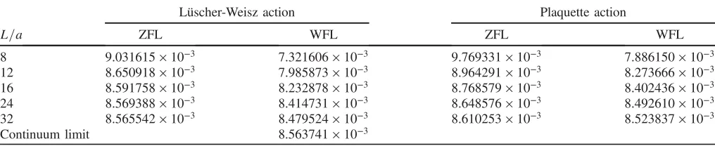
[28]. We use the nonperturbatively determined c_swðg₀Þ TABLE I. Tree-level values oft2hEmagðt; xÞiforc¼

ffiffiffiffi 8t p

=L¼0.3,x₀¼T=2and both the Oða2Þtree-level improved Lüscher-Weisz gauge action and the plaquette gauge action (cf. Sec.V). We quote the two choices of flow discretizations that we consider in this work: Zeuthen flow/Lüscher-Weisz (LW) observable (labelled ZFL) and Wilson flow/clover observable (labelled WFL). See Sec.IIIfor more details. The continuum valueNðcÞis also reported.

Lüscher-Weisz action Plaquette action

L=a ZFL WFL ZFL WFL

8 9.031615×10−3 7.321606×10−3 9.769331×10−3 7.886150×10−3 12 8.650918×10−3 7.985873×10−3 8.964291×10−3 8.273666×10−3 16 8.591758×10−3 8.232878×10−3 8.768579×10−3 8.402436×10−3 24 8.569388×10−3 8.414731×10−3 8.648576×10−3 8.492610×10−3 32 8.565542×10−3 8.479524×10−3 8.610253×10−3 8.523837×10−3

Continuum limit 8.563741×10−3

[29]. Except at the time boundaries, our action is the same as the one used by the CLS Collaboration[15].

With our choice of boundary conditions in time, the complete removal of OðaÞeffects requires the knowl-edge of the boundary improvement coefficientsc_t, c~_t. We use their values determined in perturbation theory. For an estimate of the uncertainty of perturbation theory, we use the last known term in the perturbative series, the one-loop term (cf. Sec.III A). Details will be discussed later.

SF boundary conditions on the lattice are imposed in complete analogy to the continuum counterparts. The gauge links obey

UkðxÞjx0¼0;T ¼1; k¼1;2;3; ð2:14Þ

while the fermion boundary conditions remain the same as in the continuum, Eq.(2.3).

There is much freedom when translating the GF equa-tion(2.4)and the energy density used to define the coupling [see Eq.(2.6)] to the lattice. Different choices differ only by cutoff effects, but these can be substantial. A popular choice is the Wilson flow (no summation overμ)

a2_ð∂tV

μðt; xÞÞVμðt; xÞ†¼−g20∂x;μSW½V;

V_μð0; xÞ ¼U_μðxÞ; ð2:15Þ

where V_μðt; xÞ are the links at positive flow time and ∂x;μSW½Vis the force deriving from the Wilson plaquette gauge action [i.e. Eq. (2.8) with the choices c₀¼1, c₁¼0]. It has been shown[30]that this choice introduces Oða2Þ cutoff effects when integrating the flow equation. They can be avoided by using the Symanzik Oða2Þ improved“Zeuthen flow”equation (no summation overμ)

a2_ð∂

tVμðt; xÞÞVμðt; xÞ†¼−g20

1þa2

12Δμ

∂x;μSLW½V;

V_μð0; xÞ ¼U_μðxÞ; ð2:16Þ

where∂x;μSLW½Vis the force deriving from the Symanzik tree-level improved (Lüscher-Weisz) gauge action Eq.(2.8)

(see Ref. [30] for more details). We insert the correction termΔ_μ¼∇_μ∇_μinto the flow equation for all linksðx;μÞ except for those linksðx;0Þwhere an end point touches one of the SF boundariesx₀¼0,T. For those links, we simply set Δ₀¼0.

The discretized observable is defined as the spatial part of the Lüscher-Weisz action density, cf. Eq. (2.8). Our choices guarantee that, neglecting small terms coming from the time boundaries atx₀¼0,T, neither the gradient flow nor the definition of the observable introduce any Oða2Þ cutoff effects. The remaining cutoff effects in our flow quantities are hence produced by our lattice action Eqs. (2.8) and (2.10) and by the initial condition for the flow equation att¼0[30]. Although this is our preferred

setup, in several parts of the work, we will compare the results with the more standard Wilson flow/clover-observ-able discretization.

At nonzero a=L, our coupling definition reads

¯ g2

GFðLÞ ¼g¯20.3ðLÞ; ð2:17Þ

with

¯ g2

cðLÞ ¼t2Nˆ−1ðc; a=LÞh

Emagðt; xÞδˆðQÞi

hδˆðQÞi

ffiffiffi

8t

p

¼cL;x0¼T=2 ;

ð2:18Þ

and

E_magðt; xÞ ¼1

4½Gaijðt; xÞGaijðt; xÞLW: ð2:19Þ

Several comments are in order. We have chosen to define the coupling through just the magnetic partEmagofEsince this choice has a lower sensitivity to the boundary improve-ment coefficient ct and because its (tree-level) Oða2Þ improvement does not need any further terms.4 As in Ref.[12], the normalization factorNˆ ðc; a=LÞis computed on the lattice with our choices of discretization (action, flow, and observable), such that in the relation g¯2_GF¼ g2

0þOðg40Þthe leading term has all lattice artifacts removed (see Table I). Due to the fact that we use a tree-level improved action, and neither the Zeuthen flow equation nor the Lüscher-Weisz observable discretization introduces any Oða2Þartifacts, we furthermore have

δðc; a=LÞ≡Nˆðc; a=LÞ

NðcÞ −1¼Oðða=LÞ4Þ; ð2:20Þ

i.e. the lattice normalization in fact only corrects subleading Oðða=LÞ4Þterms. Finally, on the lattice, one has to clarify what is meant by projecting to zero topology. We define the topological charge by[9]

Q¼ 1

32π2 X

x

ϵμνρσ½Gaμνðt; xÞGaρσðt; xÞcl; ð2:21Þ

using the clover discretization of the field strength tensor of V. We then set pffiffiffiffi8t¼cL with c¼0.3 and use the Zeuthen flow. With this definition, the topological charge is not integer valued but approaches integers close to the continuum limit. Therefore, the Kronecker δQ;0 of the continuum definition is replaced by

ˆ

δðQÞ ¼

_1;

if jQj<0.5

0; otherwise: ð2:22Þ

III. GENERAL CONSIDERATIONS ON THE CONTINUUM LIMIT OF FLOW QUANTITIES

All studies of finite size scaling with the GF scheme show significant cutoff effects in the extrapolations of the step scaling function (see Ref.[10]and references therein). In fact, one may be concerned not only by the leading5 Oða2Þ effects but also by the subleading higher order corrections [in the present case, starting at Oða3Þ] that might lead to the wrong continuum limit.

Local composite fields constructed from the flow field have a natural length scale given by the smoothing radius_ffiffiffiffi

8t

p

, which is smaller than L by a factor c. Hence, the natural expansion parameter for the cutoff effects is ϵ¼a=pffiffiffiffi8t¼a=ðcLÞ. A first example is provided by checking the effects at tree level. This just amounts to studying δðc; a=LÞ, Eq. (2.20). In order to get a more general picture, we consider besides our discretization of the gradient flow and the observable (“Zeuthen flow”for short) also the one used in many studies: Wilson flow and clover discretization of the energy density [9] (for short

“Wilson flow”). We find that

δðc; a=LÞ∼

_{−0.9118ϵ2þ0.4867ϵ4}

Wilson flow 1.7165ϵ4 Zeuthen flow; ϵ¼ a

cL¼ a

ffiffiffiffi 8t

p ; ð3:1Þ

where ∼ holds with corrections of less than 10−4 for ϵ<0.33 and for c in a range 0.1–0.4. One may also consider the GF coupling for twisted periodic boundary conditions [13]; the above numbers hardly change. This example not only shows that in fact the cutoff effects are predominantly a function of ϵ¼a=pffiffiffiffi8t but also that the contribution of orders higher thanϵ2are only at the level of a few percent forϵ<0.3. There is a clear hierarchy of the different orders at smallϵ, say ϵ<0.3.

Of course, one has to study the situation beyond tree-level perturbation theory, and in particular the scaling properties of the lattice approximation to the step scaling functionσðuÞof Eq.(1.1). In order to do so, it is useful to consider the general ratio

Rc;c0ðu; a=L; sÞ ¼ g¯ 2

cðLÞ

¯ g2

c0ðsLÞ ¯

g2_cðLÞ¼u

; ð3:2Þ

that has a natural expansion

R_c;c0ðu;a=L; sÞ ¼R_c;c0ðu;0; sÞf1þA_c;c0ðuÞ½ϵ2−ϵ02 þ…g;

ð3:3Þ

whereϵ¼a=ðcLÞ andϵ0¼a=ðc0sLÞ. The connection to the standard step scaling function isσðuÞ ¼u=R_c;cðu;0;2Þ. It is again worthwhile to first consider tree level. To this end, we temporarily replace the normalizationNˆðc; a=LÞ by the continuum one, N, in Eq. (2.18); otherwise, all cutoff effects are removed. With this replacement, the tree-level ratioR_c;c0ðu;0; sÞis to a very good approximation just a function of u and the product sc0, while the function A_c;c0ðuÞ _{depends little on} c, c0_{. An inspection of our} numerical data shows that this is true also at nonvanishing coupling. These properties allow us to gain insight into the scaling properties of the step scaling function by consid-ering the cases¼1where we can use our full data set. As we shall see in Sec. IV, we have five lattice resolutions L=a¼8, 12, 16, 24, 32 at our disposal. Continuum extrapolations can involve a change of the lattice spacing of up to a factor 4. Moreover, these ratios can be computed even more precisely than the step scaling function, since they are evaluated on the same ensembles and one benefits from the statistical correlation of the data.

Figures 1 and 2 show Rc;c0ðu; a=L;1Þ _{for all together} six different combinations, c, c0, and two values of u. The data originate from the simulations described in Appendix, forming first the ratios at the availableg¯2_c and then performing a (very smooth) interpolation to the two chosen values of u. As shown in the figures, we separately extrapolate the ratios for the two different discretizations of the flow observables to the continuum limit. We use a purea2ansatz for the cutoff effects in the ranges

FIG. 1. RatioR₀.3;c0ð4.26; a=LÞfor variousc0and two different discretizations of the observable. In the definition Eq.(3.2), all quantities refer to the same discretization. Full lines are linear fits ina2 to data satisfying Eq.(3.4).

jϵ2_−ϵ02_{j ¼ j1−ðc}0_=cÞ2_j

_a

c0_{L 2}

< ₀

.10 Wilson flow; 0.25 Zeuthen flow:

ð3:4Þ

The data are compatible with the linear behavior in a2, and the so-estimated continuum limits agree. The test is rather stringent because here the precision is higher than in the step scaling functions, which form the core observables of the rest of this paper. For the step scaling functions, there is no analogy of the correlations of the numerator and denominator in Eq. (3.2), which enhance the precision ofR_c;c0ðu; a=L;1Þ. Figure1and Fig.2are a good confirmation that higher order cutoff effects are small, when Eq. (3.4) is satisfied.

Translating the bounds (3.4) to the case of the step scaling function, we have

½1−ð1=2Þ2

a cL

₂ <

₀

.10 Wilson flow;

0.25 Zeuthen flow: ð3:5Þ

We then expect the step scaling function computed using the Zeuthen flow to have only small corrections to an a2 scaling forϵ2¼a2=ðcLÞ2<0.33. Our coarsest data set has L=a¼8 andc¼0.3, which impliesϵ2¼0.17.

The difference in the bounds(3.5)means that the more precise continuum limit is obtained for the Zeuthen flow. Despite the fact that cutoff effects for the Wilson flow are smaller, their complicated functional form makes extrap-olations more difficult and less precise. In particular, the coarser lattices used to determine the continuum step scaling function in the next section would have significant violations of the leading a2 scaling if we were using the Wilson flow data.

However, one has to state that the a2 corrections are sizable. Since neither the Zeuthen flow equation nor the evaluation of a classically improved observable introduces anya2cutoff effects, these remaining lattice artifacts are a consequence of the quantum corrections due to the initial condition of the flow equation att¼0and due to the action of the fluctuating fields in the path integral[30]. Whether there are practical ways to reduce these remaininga2effects substantially is an interesting problem that deserves further attention in the future.

A. BoundaryOða=LÞeffects

With our choice of SF boundary conditions(2.14),(2.3), the complete removal of OðaÞ cutoff effects requires not only the nonperturbative value of the coefficientcsw [29] but also the determination of the boundary coefficientsct, ~

c_t[4,28]. These are known only to one loop for our choice of lattice action[31–33]

c_t¼1þcð_t1Þg2

0þOðg40Þ; cðt1Þ¼0.0326718; ~

c_t¼1þc~ð_t1Þg2

0þOðg40Þ; c~tð1Þ¼−0.01505; ð3:6Þ

and therefore we have to estimate the possible effects of higher order terms in the coupling.

For this purpose, it is convenient to recall that our GF coupling is defined at time slice x₀¼T=2, and with our choice_ffiffiffiffi c¼0.3 and T ¼L, the smearing radius is

8t

p

¼cL¼0.3T. Therefore, we expect boundary effects to be suppressed, since our observable is localized at the center of the lattice, away from the boundaries. The issue was investigated in Ref. [14] with the conclusion that indeed these boundary contributions are small. Here, we estimate the effect quantitatively and specifically for our observable.

We first quote the linear a-effects at leading order in perturbation theory. They are obtained by expanding the tree-level normN in ct−1, treatingct¼1þOðg20Þ. The result is

Σðu; a=LÞ ¼Σðu; a=LÞ_ct¼1þct−1 g2

0cðt1Þ

ΔctΣðu; a=LÞ; ð3:7Þ

ΔctΣðu; a=LÞ ¼rð1Þ

1 Σ2 a

2LþOðΣ3Þ; ð3:8Þ

withrð₁1Þ ¼−0.013in the relevant range ofL=a≥8. We have normalized by the one-loop contribution toct, using the knowncð_t1Þ. In this way,ΔctΣ_{gives the effect in}Σ_{if one}

takes as an uncertainty the one-loop term in the perturbative series ofct. As here the one-loop term is the last known one, this is exactly what we want to do in this work.

As a check on the use of perturbation theory, we performed simulations on our smallest latticeL=a¼8 at FIG. 2. RatioR₀.36;c0ð8.24; a=LÞfor variousc0and two different

¯

g2_{∼4.5 with three different values ofc}

t around the one-loop one. We found that the effective coefficient

reff 1 ≡2

L a Σ−2

∂Σ ∂ct

ð3:9Þ

evaluates to

reff

1 ¼−0.0121ð5Þ g2

0cðt1Þ

Σ2 ð3:10Þ when we estimate it from a numerical derivative at our central simulation point c_t¼1þcð_t1Þg2₀. The agreement with lowest order perturbation theory is good enough to just take Eq.(3.7) as our estimate of the uncertainty.

We propagate (by quadrature) the full one-loop effect of this boundary counterterm (3.7) to our error on Σðu; a=LÞ. Note that this effect is subdominant in comparison with our statistical accuracy. The correspond-ing uncertainty due to c~t will be neglected since it is suppressed by a further power of g2.

IV. CONTINUUM EXTRAPOLATIONS

AND THE β-FUNCTION

As already mentioned, the way to connect nonperturba-tively the hadronic scaleL_hadand the intermediate scaleL₀ passes through the computation of the step scaling function. It is defined as the continuum limit

σðuÞ ¼ lim

a=L→0Σðu; a=LÞ ð4:1Þ

of its lattice approximation,

Σðu; a=LÞ ¼g¯2

GFð2LÞjg¯2_GFðLÞ¼u;m¼0: ð4:2Þ

The condition m¼0 fixes the bare quark mass for each resolutiona=Land each value of the bare couplingg2₀. The resulting function is denotedmcrðg0; a=LÞand described in Appendix. The second condition,g¯2_GFðLÞ ¼u, fixesg₀for each value of u and resolution a=L considered. The doubled lattices, where g¯2_GFð2LÞ is determined, share the bare parameters with theL=alattices.

A. Strategy and data set

In practice, these conditions have to be implemented by a tuning of the bare parameters such that the renormalized ones are fixed as described. We briefly explain our strategy to arrive at a precise tuning for a few appropriate values ofu and the estimates ofΣ:

(i) The tuning of the bare massm₀was already carried out in Ref.[33]for the full range of bare couplings and a=L considered. In the continuum limit, the chiral point of vanishing quark mass is unique; the a=L-dependence is a cutoff effect. However, in order to have a smooth extrapolation to the continuum limit,

one first defines exactly which mass is set to zero at a fixed a=L and then determines the function mcrðg0; a=LÞ. In the cited reference, this task was carried out with high precision. As a result, we can neglect any deviations from the exact critical line. The used functionsmcrðg0; a=LÞare listed in Appendix. (ii) For the next step, we performed nine precise simulations with L=a¼16. These determine nine values ofu¼vi; i¼1;…;9, which we take as our

prime targets to compute σðviÞ. We further need

values of β for L=a¼8, 12 such that g¯2_GF equals our target values v_i. This is achieved by an inter-polation of several simulations described in detail in Appendix B. At this point, we found for each L=a¼8, 12, 16 nine values of β where couplings ¯

g2

GFðLÞmatch rather well. Theseβ-values are listed in TableII.

(iii) We then carried out simulations on the doubled lattices at the same values ofβ,m₀; see columns 4–6 in Table II. The data for g¯2_GFð2LÞ in the table are estimates of the step scaling functionΣðu; a=LÞ at u¼g¯2

GFðLÞβ;L=a. For our estimates for g¯2GFðLÞ, we could take the numbers from the interpolation in step 2. These are simply the same as those at L=a¼16. However, in order to enhance the pre-cision, we perform separately at eachL=a¼8, 12 an interpolating fit to all available data of TableIX. These fits determineg¯2_GFðLÞ in TableII. Details on the very well-determined interpolation are given in AppendixB.

(iv) For the last step, we propagate the errors ofg¯2_GFðLÞ into those ofΣ. As we will see in Sec.IV B 1, our nonperturbative data are well described by the functional form

1 Σ−

1

u¼constant; ð4:3Þ

which suggests using the derivative, ∂Σ=∂u¼ Σ2_=u2_{, for the error propagation. This yields the} last column of TableII, whereuis the central value ofg¯2_GFwithout error. The difference of the errors in columns 4 and 7 is mostly due to the uncertainty of OðaÞ improvement, Eq. (3.7); a small part of the uncertainty is also contributed by the propagated errors of g¯2_GFðLÞ.

The last two rows in Table II are from additional simulations performed with the aim of having ¯

g2

GFð2LÞ≈11.3. They will also be useful below.

B. Continuum extrapolation of the step scaling function

However, our investigation in Sec. III showed that the cutoff effects are strongly dominated by theða=LÞ2terms, which motivates extrapolations linear in this variable.

Given the high precision which we achieve, this is a crucial part of this work, and a detailed analysis will follow. In particular, we first study the systematic effects in the continuum determination of σðuÞ by performing inde-pendent extrapolations at nine fixed values ofu. These can transparently be illustrated by simple graphs.

1.σðuÞ and systematic effects in the continuum extrapolations

Apart from the last two rows of TableII, the deviations of ¯

g2

GFðLÞ from the nine target values vi (the ones at L=a¼16) are very small. We can therefore simply shift the data forΣusing Eq.(4.3). The resulting data are shown in Fig.3. Within the uncertainties, linearity ina2is perfect, and we extrapolate by

TABLE II. Step scaling functions. At the specifiedβ, we listg¯2ðLÞon theL=a-lattice obtained from the described fit as well asg¯2ð2LÞ on the2L=a-lattice. Their errors do not contain the uncertainty ofct.Nms and NQ refer to the measurements on the2L=a-lattice Simulations with NQ¼∅were carried out with the algorithm restricted to Q¼0. Atβ¼3.556470 and L=a¼16, we have two

ensembles, with and without fixing the topology (both ensembles give compatible results, and in columns 4 and 7, we quote as results the weighted average). The last column containsΣðu; a=LÞwithuequal to the central value of column 3 and the full error obtained from ¯

g2_ðLÞ,g¯2_{ð2LÞas well as the uncertainty ofc}

t. Note that errors in columns 3 and 7 are correlated, as discussed in the text.

L=a _β g_¯2_{ðLÞ g¯}2_{ð2LÞ N}

ms NQ Σðu; a=LÞ

8 3.556470 6.5485(60) 11.452(79) 2000, 2000 725;∅ 11.452(134)

8 3.653850 5.8670(34) 9.250(66) 2000 220 9.250(97)

8 3.754890 5.3009(32) 7.953(44) 2001 30 7.953(68)

8 3.947900 4.4848(25) 6.207(23) 2001 1 6.207(39)

8 4.151900 3.8636(21) 5.070(16) 2001 0 5.070(26)

8 4.457600 3.2040(18) 3.968(11) 2001 0 3.968(17)

8 4.764900 2.7363(14) 3.265(8) 2001 0 3.265(12)

8 5.071000 2.3898(15) 2.772(6) 2001 0 2.772(9)

8 5.371500 2.1275(15) 2.423(5) 2001 0 2.423(7)

12 3.735394 6.5442(82) 12.874(165) 3000 ∅ 12.874(191)

12 3.833254 5.8728(46) 10.497(78) 2400 ∅ 10.497(99)

12 3.936816 5.2990(36) 8.686(49) 2400 ∅ 8.686(64)

12 4.128217 4.4908(32) 6.785(36) 2400 1 6.785(44)

12 4.331660 3.8666(25) 5.380(25) 2400 0 5.380(29)

12 4.634654 3.2058(17) 4.180(14) 2403 0 4.180(17)

12 4.938726 2.7380(15) 3.403(11) 2400 0 3.403(13)

12 5.242465 2.3902(11) 2.896(9) 2400 0 2.896(10)

12 5.543070 2.1235(12) 2.504(8) 2400 0 2.504(9)

16 3.900000 6.5489(155) 13.357(136) 1205 ∅ 13.357(167)

16 4.000000 5.8673(140) 10.913(118) 1404 ∅ 10.913(136)

16 4.100000 5.3013(134) 9.077(75) 1403 1 9.077(91)

16 4.300000 4.4901(77) 6.868(40) 2507 0 6.868(48)

16 4.500000 3.8643(63) 5.485(22) 2000 0 5.485(28)

16 4.800000 3.2029(52) 4.263(16) 2000 0 4.263(20)

16 5.100000 2.7359(35) 3.485(11) 2500 0 3.485(14)

16 5.400000 2.3900(30) 2.935(7) 2500 0 2.935(9)

16 5.700000 2.1257(25) 2.536(7) 2500 0 2.536(8)

12 3.793389 6.1291(56) 11.788(132) 2556 ∅ 11.788(154)

16 3.976400 6.037(14) 11.346(100) 1203 ∅ 11.346(124)

Σðvi; a=LÞ ¼σiþr~i×ða=LÞ2; ð4:4Þ

at each valuev_i. The quality of the fits is very good with a totalχ2of 6.3 with 9 degrees of freedom. The fit parameters σi, second column of Table III, are first estimates of the

continuum step scaling function. It turns out that the nonperturbative results are well described by1=σi−1=vi≈ −0.083(see the last two columns of TableIII), which is the functional form of one-loop perturbation theory, but with a coefficient slightly different from the perturbative−0.0790. This surprising behavior holds out to σðuÞ ¼Oð10Þ. We will come to a comparison with perturbation theory later. For now, this suggests fitting also

1=Σðvi; a=LÞ ¼1=σiþri×ða=LÞ2: ð4:5Þ

The quality of these fits is as good as the previous ones (χ2¼6.3 for 9 degrees of freedom). Discriminating sta-tistically between the two fit forms would require far higher precision than we have.

An implicit assumption behind Eq.(4.4)and(4.5)is that higher orders ina2are negligible. When this is the case, the fit parameters σ_i have to agree between the two fits (see Table III). There is agreement at the level of one standard deviation. However, the difference between the two extrapolations is of course systematic:σiare always larger

when they are extrapolated following Eq.(4.5). This is also apparent in Fig.3. Furthermore, when nonlinearities ina2 are negligible, there is the more stringent condition ri¼−r~i=σ2i. As expected, we find more significant

differences between these slope parameters6 (see Fig. 4).

Note that the difference between the functional forms of Eq.(4.4)and Eq.(4.5)is of ordera4. Due to the relatively large Oða2Þeffects, these are not negligible at large values of the coupling (at small values ofu, we have good agreement between both types of fits). It is this Oða4Þ effect that produces a systematic shift in the parametersσi,ri.

A fit of 1=σðuÞ−1=u to a constant provides a good description of our continuum data (χ2=dof<1) in the whole rangeu∈½2.1;6.5. Although the systematic differ-ence between the continuum fits(4.4)and(4.5)was point by point inσibelow our statistical accuracy, the uncertainty

in a constant fit to1=σðuÞ−1=uis reduced by a factor 3 due to the fact that we use nine independent values to determine it. The systematic effect then becomes clearly noticeable.

2. Fitting strategy

The previous considerations illustrate that the Oða4Þ effects are not large but still cannot simply be ignored. The size of the Oða2Þterm, that amounts to 20% at the largest value of the couplingu_max¼6.5atL=a¼8, suggests that there the Oða4Þeffects are around 5%. Taking into account that au-independent term is removed by the normalization of the coupling, this translates into the rough scaling

Δsys_Σ

i¼0.05Σi

8_La

_{4 u}

umax

: ð4:6Þ

This systematic effect is negligible compared with our statistical accuracy for the lattices with L=a≥12 at all values ofu(in fact, the differences seen in TableIIIbecome insignificant when we perform the extrapolations with just L=a≥12), but it becomes dominant atL=a¼8and large values ofu.

When fitting to some particular functional form, one performs a minimization of aχ2 function, defined as TABLE III. Examples for the continuum limits of the step

scaling function σi¼lima=L→0Σðvi; a=LÞ obtained by various

extrapolations at fixed values ofu¼vi. The last row shows fits of

columns 4 and 5 to a constant. These fits to a constant provide an excellent description of our data.

σi ð1=σi−1=viÞ×102 v_i Eq.(4.4) Eq.(4.5) Eq.(4.4) Eq. (4.5)

6.5489 14.005(175) 14.184(197) −8.13ð10Þ −8.22ð12Þ 5.8673 11.464(123) 11.654(146) −8.32ð10Þ −8.46ð13Þ 5.3013 9.371(79) 9.468(89) −8.19ð11Þ −8.30ð12Þ 4.4901 7.139(47) 7.181(51) −8.26ð11Þ −8.34ð12Þ 3.8643 5.622(28) 5.641(30) −8.09ð10Þ −8.15ð14Þ 3.2029 4.354(19) 4.367(21) −8.25ð12Þ −8.32ð13Þ 2.7359 3.541(14) 3.550(15) −8.31ð12Þ −8.38ð13Þ 2.3900 2.991(10) 2.996(10) −8.40ð12Þ −8.46ð13Þ 2.1257 2.575(9) 2.578(9) −8.21ð14Þ −8.26ð14Þ

Constant fit: −8.233ð37Þ −8.316ð42Þ FIG. 4. Slopesriof Eq.(4.5)and−~ri=σ

2

i withr~i of Eq.(4.4).

6_{Note that the determination of asymptotic values ofr}

iorr~iis

χ2_ðp αÞ ¼

XNdata

i¼1

W_i½fðx_i;p_αÞ−y_i2_{; ð4:7Þ}

where p_α represent the parameters that describe the function fðx_i;p_αÞ and x_i, y_i are the independent and dependent variables, respectively. The weight,Wi, of each

data point is usually taken from their uncertainty, but here we should take into account that we cannot expect our data to be more accurately described by a linear function ina2 than Δsys_Σ

i. For the following, we therefore define the

weights by

W−1

i ¼ ðΔΣiÞ2þ ðΔsysΣiÞ2; ð4:8Þ

which strongly reduces the weights of the points further away from the continuum. Note that we distinguish the weights of the fits from the errorsΔΣiof the data (statistical

and the one due to the uncertainty in ct), which enter the error propagation from the data to the parameters of the fit. For an example for the consequences of introducingW_i, we repeat fits(4.4)and(4.5). We obtain continuum values 1=σðuÞ−1=u which are still perfectly described by a constant, but now the values of the constants are

−0.0824ð5Þand−0.0830ð6Þ, respectively. Comparing with the last row of Table III, we see that uncertainties have increased and central values are closer. Now, both types of fits agree within one standard deviation.

3. Determination ofσðuÞ

As already noted, our nonperturbative data are very well described by an effective one-loop functional form. This suggests two strategies to determine the continuum step scaling function. First, we can perform continuum extrap-olations at constant values ofuas suggested in the previous sections [Eq.(4.4)and Eq.(4.5)]. The continuum values of σðv_iÞ can then be fitted to a functional form,

1 σðviÞ−

1

vi¼QðviÞ; QðuÞ ¼

X

n_σ−1

k¼0

c_kuk_{: ð4:9Þ}

The number of parametersn_σis varied in order to check the stability of the procedure. Second, one can also consider the possibility of combining the ansatz for the cutoff effects immediately with the parametrization of the continuum functionσðuÞ,

1 Σðu; a=LÞ−

1

u¼QðuÞ þρðuÞða=LÞ2: ð4:10Þ

Apart from checking the stability of the procedure, advan-tages of this global fit are as follows. The shifts to common values ofufor differenta=Lare not needed, and the data in the last two rows of TableIIare easily included. Also, more general forms of cutoff effects can be tried. Our inves-tigation suggests that

ρðuÞ ¼X n_ρ−1

i¼0

ρiui ð4:11Þ

is a good parametrization ofρwhen at leastn_ρ¼2terms are included.

Figure 5 shows a comparison between the individual extrapolations at fixeduaccording to(4.4)and(4.5), and a global fit(4.10)withn_σ ¼n_ρ¼2. We recall that all fits are performed with the weights of Eq.(4.8).

A more quantitative test of the agreement between theσ obtained from different analysis is through the sequence u₀¼11.31,u_i≥1, Eq.(1.4). We collect this information in Table IV. Once the polynomial is not too restricted, the results depend very little on the number of termsn_σ since we use this polynomial interpolation only in the range where data are available.

C. Determination of theβ-function

Since our main goal is the determination of the scale factor Lhad=L0 [see Eq. (1.6)], it is very convenient to replace the parametrization ofσðuÞby a parametrization of theβ-function. Namely, we write

βðgÞ ¼−_Pðg_g3_2Þ;

Pðg2_{Þ ¼p}

0þp1g2þp2g4þ…: ð4:12Þ

The one-loop effective β-function just corresponds to the choice PðuÞ ¼p₀, while higher order terms parametrize possible (obviously small) deviations useful for a more detailed analysis and an estimate of uncertainties. The step scaling function is then given by

logð2Þ ¼−

Z ffiffiffiffiffiffiffip_σðuÞ ffiffi

u

p

dx βðxÞ¼

Z pffiffiffiffiffiffiffi_σðuÞ ffiffi

u

p dx

Pðx2_Þ x3

¼−p0

2

1 σðuÞ−

1 u

þp1

2 log

σðuÞ

u

þX

nmax

n¼1 pnþ1

2n ½σnðuÞ−un; ð4:13Þ

where n_σ parameters correspond to n_max¼n_σ−2. The parameters pi, i¼0;…; nσ−1, in Eq. (4.12) can be obtained by fitting our data for σðuÞ to Eq. (4.13). Any of our previous methods to extrapolate the lattice step scaling functionΣðu; a=LÞto the continuum can be used. In the case of the global fits, we make use of a further variant to parametrize the cutoff effects by fitting

logð2Þ þρ~ðuÞða=LÞ2¼−

Z pffiffiffiffiffiffiffiffiffiffiffiffiffiffi_Σðu;a=LÞ ffiffi

u

p

dx

βðxÞ: ð4:14Þ

Note that this fit ansatz differs from other global fits only by terms Oða4Þ. Comparing the different approaches provides an additional check that these effects are under control (see discussion in SectionsIV B 1 andIV B 2).

Solving numerically Eq.(4.13)foru, we then compute the series of couplings ui. In Table IV, we compare the

results to those obtained via the parametrizations of the step scaling function. There is good agreement between differ-ent types of fits.

Figure6shows a comparison of theβ-function obtained with two different fits. Their agreement underlines that all uncertainties have been taken care of and that the small

difference to the one-loop β-function is significant. The difference to the universal two-loop β-function is even larger in the region of g2≳3. Therefore, perturbation theory is of little use in our range of couplings.

In the following, we will use as our central result and uncertainty the fit in the last row of the table. It has the largest uncertainties and parameters

p₀¼16.26ð69Þ; p₁¼0.12ð26Þ;

p₂¼−0.0038ð211Þ; ð4:15Þ

with covariance matrix

covðp_i;p_jÞ

¼

0 B @

4.78071×10−1−1.76116×10−1 1.35305×10−2

−1.76116×10−1 6.96489×10−2−5.54431×10−3 1.35305×10−2_{−5.54431×10}−3 _4.54180×10−4

1 C A:

ð4:16Þ

V. CONNECTION OF SCALES 1=L₀ AND 1=L_had

A. Matching with the scale 1=L₀

In this section, we relate the scale 1=L₀ defined in Ref.[1] by the condition

¯ g2

SFðL0Þ ¼2.012; ð5:1Þ

to the coupling in our GF scheme. More precisely, we define the function

φðuÞ ¼ lim

a=L→0Φðu; a=LÞ; ð5:2Þ TABLE IV. Coupling sequence Eq.(1.4)withu₀¼11.31and scale factorssðg2₁; g2₂Þforg2₁¼2.6723,g2₂¼11.31for different fits to cutoff effects and the continuum β-function. Fits are labelled by Σor1=Σfor continuum extrapolations according to Eq. (4.4)or Eq. (4.5), respectively, while the parametrization of the continuum step scaling function is labelled as σ for σðuÞ ¼uþs₀u2þ

s₁u3_þu3Pnσ

n¼1cnunand labelled asQfor Eq.(4.9). Fits to theβ-function [Eq.(4.12)] are labelledP. For global fits, we specifynρ, of Eq.(4.11), while its absence indicates a fit of data extrapolated to the continuum at each value ofu¼v_i. The weightsW_irefer to the definition of χ2, Eq.(4.7).

Fit n_σ n_ρ Wi u1 u2 u3 u4 sðg21; g22Þ

Σ;_σ 3 – ΔΣ−_i2 5.866(21) 3.955(17) 2.981(13) 2.392(11) –

Σ,Q 3 – ΔΣ−_i2 5.867(21) 3.956(16) 2.981(14) 2.391(12) –

1=_Σ,Q 3 – ΔΣ−_i2 5.832(21) 3.927(17) 2.960(13) 2.374(11) –

1=_Σ,P 2 – ΔΣ−_i2 5.832(21) 3.927(15) 2.959(13) 2.374(11) 10.82(14)

1=_Σ,P 3 – ΔΣ−_i2 5.831(21) 3.926(17) 2.959(13) 2.374(11) 10.82(15)

Σ,P 3 – (4.8) 5.870(28) 3.954(22) 2.976(17) 2.385(15) 11.00(20) 1=_Σ,P 1 3 (4.8) 5.843(20) 3.939(18) 2.971(16) 2.385(13) 10.96(18) 1=_Σ,P 2 3 (4.8) 5.864(26) 3.944(19) 2.968(16) 2.378(14) 10.90(18) 1=_Σ,P 3 3 (4.8) 5.864(27) 3.944(21) 2.968(17) 2.378(14) 10.90(19) (4.14),P 2 2 (4.8) 5.872(27) 3.949(19) 2.971(16) 2.379(14) 10.93(19) (4.14),P 3 3 (4.8) 5.874(28) 3.951(22) 2.972(17) 2.379(14) 10.93(20)

with

Φðu; a=LÞ ¼g¯2

GFð2LÞj¯g2_SFðLÞ¼u;m¼0: ð5:3Þ

Recall that the SF coupling is defined with a background field, while the boundary conditions of our gradient flow scheme correspond to a zero background field. The con-nection between the couplings goes through the common bare parameters defined by the condition g¯2_SFðLÞ ¼u, m¼0, together with the resolutiona=L.

We do not need the functional dependence on u, but rather just the single value φð2.012Þ. We combine the change of schemes SF→GF with a scale change by a factor of 2, because this avoids the disadvantages of both schemes at the same time:g¯2_GFhas noticeable cutoff effects whena=Lis too small, andg¯2_SFneeds very large statistics if L=ais too large. A last choice to make is the discretization. Here, we choose the Wilson gauge action where the counterterms (coefficientsc_t,c~_t; see Ref.[1]) which cancel linearaeffects are perturbatively known, such that they are suppressed to the negligible level ofg8a=L. The action as well as the definition of the critical linem¼0is exactly as in Refs.[1,34]. In fact, with the exception ofL=a¼16, the numerical values of β, κ, g¯2_SF in Table Vare taken from there, interpolated to the fixed value g¯2_SF¼2.012. More details will be given elsewhere[34]. Our measurements of the GF coupling on the doubled lattices (Zeuthen flow) are listed in TableV. The errors in the last column include the errors ofg¯2_SFðL₀Þ(column 4 of TableV). Like for the step-scaling function in Eq. (4.3), we use the derivative ∂uΦðu; a=LÞ≃Φðu; a=LÞ2_=u2 _{for the Gaussian error} propagation. The additional error does not depend very much on this particular ansatz and is subdominant, as can be also seen in TableVand in Fig.7where the errors both before and after error propagation are shown.

The continuum extrapolation ofΦcan be seen in Fig.7. We also show results with the Wilson flow, but the Zeuthen flow(2.18)has smaller cutoff effects. Due to the very high statistical correlation of the numbers, a combination of the two discretizations of the flow observable does not lead to an improvement of the final errors. We therefore quote only the continuum limit from the Zeuthen flow. The main result of this section is then

¯ g2

GFð2L0Þ ¼φð2.012Þ ¼2.6723ð64Þ: ð5:4Þ

B. Ratio L_had=L₀

Using our fits to the β-function, the scale factor s¼ L₂=L₁ betweeng₂¼g¯ðL₂Þandg₁¼g¯ðL₁Þcan be easily computed via

logðsðg2₁; g2₂ÞÞ ¼ Z _g

2

g1

dxPðx2Þ x3 ¼

p₀ 2g2

1− p₀ 2g2

2

þp₁log _g

2 g₁

þX

nmax

n¼1 p_nþ1

2n ½g22n−g21n: ð5:5Þ

Numbers forsfrom the various fits are shown in the last column of TableIV. They refer to our default value g2₂¼ ¯

g2

GFðLhadÞ ¼11.31 defining Lhad and g2₁¼g¯2GFð2L0Þ ¼ 2.6723given by the central value ofφð2.012Þdetermined above. The error ofφcan be propagated straightforwardly, yielding

Lhad=L0¼21.86ð42Þ: ð5:6Þ

AsΛð3Þ

MS¼0.0791ð21Þ=L0is known[1], the last step on the way to a determination of theΛ-parameter in physical units is the computation of a physical observable of dimension mass in large volume and at the physical masses of the three quarks. This has to be combined withLhad=a at identical bare couplings and extrapolated toa¼0. Passing this last milestone still needs input from the CLS ensembles[15]. FIG. 7. Continuum extrapolation of g¯2GFð2L0Þ with the bare parameters determined by the condition g¯2_SFðL₀Þ ¼2.012. The continuum extrapolation is performed using both the Wilson flow/clover discretization and our preferred setup Zeuthen flow/ LW observable (the latter shows smaller discretization effects). The two types of error bars for each data point correspond to the inclusion or not of the propagated error for the SF coupling, cf. the text.

TABLE V. Data for both the SF and GF couplings as required for the matching procedure.

L=a _{β κ} g_¯2

SFðLÞ g¯2GFð2LÞ Φðu; a=LÞ 6 6.2735 0.1355713 2.0120(27) 2.7202(36) 2.7202(61) 8 6.4680 0.1352363 2.0120(30) 2.7003(41) 2.7003(68) 12 6.72995 0.1347582 2.0120(37) 2.6912(45) 2.6912(80) 16 6.9346 0.1344121 2.0120(17) 2.6742(65) 2.6742(72)

VI. DISCUSSION

The main goal of this work was to connect the (technical) scalesL₀andLhadprecisely. This is one of the three steps leading to a determination of the three-flavorΛ-parameter in physical units.

The precision of the result, Eq.(5.6), is rather remarkable since such a scale ratio can only be determined through the running of a coupling and a step scaling strategy[3]—at least if one wants to obtain a purely nonperturbative result and a controlled continuum limit. Since couplings usually run relatively slowly, it is necessary to determine this running with extreme precision in order to achieve the 2% accuracy on the scale ratio. Through the gradient flow [9] running coupling in a finite volume [12], we achieved excellent precision. However, scaling violations had to be dealt with very carefully. After applying systematic Symanzik improve-ment[30], they were still very significant, but we could show that they are rather accurately described by ana2behavior when the flow time,t, satisfiesa2=ð8tÞ<0.3. Since we chose our lattice spacings small enough, we could extrapolate to the continuum with three resolutions. All in all, this milestone on the way to a preciseΛ-parameter has been passed.

Let us discuss also what else we have learned on the way. The behavior of the step scaling function, Fig.5, is rather surprising. It follows the one-loop functional form very precisely, but with a coefficient slightly different from the universal perturbative one, out to large values of the coupling. For further details, one better considers the β-function (Fig. 6). Here, the nonperturbative result is in the middle between one loop and two loops at our smallest coupling, α¼g¯2_GFðLÞ=ð4πÞ ¼0.17. Describing this by higher order perturbation theory requires a large three-loop coefficient and therefore signals the breaking down of perturbation theory at this coupling or close by. One might consider the statistical significance at the weakest coupling in Fig.6insufficient for a strong conclusion, but the effect becomes increasingly significant at largerα. For example, at α¼0.25, still a coupling where perturbation theory is routinely used, the nonperturbative running is many stan-dard deviations away from two loops. Perturbation theory has broken down. This finding reinforces what we saw before in the SF schemes, where the region belowα≈0.2 was studied [1]. The β-function in one of the schemes (ν¼0) discussed in Ref.[1]is close to the known three-loop one, while other schemes are significantly off. In Fig.8, we plot it together with the GF scheme used in this paper. For the GF scheme, we show only the range of couplings covered by our data. In contrast, for the SF scheme, we show it all the way to g¼0, since the connection to the asymptotic perturbative behavior was convincingly established. The figure provides a warning that perturbation theory needs to be applied with great care in the sense that its asymptotic nature should not be forgotten. For more details, we refer to Ref.[1]. The figure also summarizes well where we stand concerning the determination of Λ. “Only” the very low energy connection of the GF scheme to the hadronic world

remains to be carried through. The CLS simulations will allow us to achieve this with an estimated 1%–1.5% precision[15,35–37]. For now, let us just mention that a combination of the rough resultg¯2_GFðLÞ ¼11forβ¼3.55, L=a¼16 with the lattice spacing of [15] yields L_had¼1fm. We have therefore computed the running in a range ofμfrom around 200 MeV to 4 GeV.

ACKNOWLEDGMENTS

We thank our colleagues in the ALPHA Collaboration, in particular C. Pena, S. Schaefer, H. Simma, and U. Wolff for many useful discussions. We would also like to show our gratitude to S. Schaefer and H. Simma for their invaluable contribution regarding important modifications to the

the Spanish MINECO’s “Centro de Excelencia Severo Ochoa” Programme under Grant No. SEV-2012-0249 as well as from Grant No. FPA2015-68541-P (MINECO/ FEDER). This work is based on previous work[38]supported strongly by the Deutsche Forschungsgemeinschaft in the Grant No. SFB/TR 09.

APPENDIX A: ALGORITHMS, SIMULATION PARAMETERS, AND AUTOCORRELATIONS

In this work, we simulated with a modified version of the openQCD v1.0 package [26], using a Hasenbusch-type splitting of the quark determinant for two of our mass-degenerate quarks [39,40] and a Rational Hybrid Monte Carlo (RHMC)[41,42]for the third one. Apart from boundary terms, we have the same action as CLS. The interested reader may find it useful to consult Ref.[15], where those simulations are described. Here, we focus on some peculiarities of our finite volume simulations: the projection to the zero topological charge sector, the scaling of the spectral gap of the Dirac operator, and the behavior of the integrated autocorrelation times of the renormalized coupling. The latter characterize the performance of the algorithm and hence the effort which we put into the computation.

1. Algorithms

An important speed up in Hybrid Monte Carlo (HMC) simulations is gained by splitting the contribution of two of the quarks, ðdetDÞ2¼detðD†DÞ, into several factors [39]

and representing each factor by a separate pseudofermion field. For our expensive simulations with L=a¼24, 32, we used three factors. More precisely, the splitting is

characterized by the mass parameters, μ₀¼0, μ₁¼0.1, andμ₂¼1.2, in the notation of Ref. [26]. Having μ₀¼0 means that twisted mass reweighting, which is also imple-mented in the package, is not used. We find that this is not necessary, as the finite volume operator D†D has a suffi-ciently stable gap. We shall show results for the gap in AppendixA 2.

A peculiar aspect of our finite volume renormalization scheme is that we are only interested in expectation values obtained in the zero topological sector [see Eq.(2.6)]. On the lattice, this is implemented by using the definition of the topological charge at positive flow time [see eqs. (2.21)– (2.22)and Ref. [43] for more information]. We explored two possibilities in order to obtain these expectation values: (i) Algorithm A:Use a standard simulation, and include the termδˆðQÞ, Eq.(2.22), as part of the definition of the observable.

(ii) Algorithm B:Include the factorδˆðQÞas part of the Boltzmann weight, and generate an ensemble that only contains configurations withjQj<0.5. This is easily implemented by adding an accept/reject step after each trajectory.

A consistency check between the two procedures was performed by generating two ensembles at L=a¼8, β¼3.556470: one with Algorithm A and a second with Algorithm B, obtaining, respectively,g¯2_GFð2LÞ ¼11.54ð11Þ andg¯2_GFð2LÞ ¼11.39ð11Þ. The average is given in TableII. In our tables, we use NQ to denote the number of

configurations that have jQj≥0.5 and therefore do not contribute to the determination of expectation values. The symbol ∅, instead, denotes an ensemble produced with Algorithm B. These ensembles havejQj<0.5throughout.

TABLE VI. Parameterradetermining the interval of the Zolotarev approximation (we always chooserb ¼7.5) and the corresponding

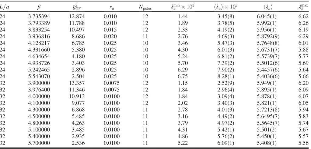
number of poles,Npoles. We also report the measured valuesλa,λb in our runs.

L=a _β g¯2

GF ra Npoles λmina ×102 hλai×102 hλbi λmaxb

24 3.735394 12.874 0.010 12 1.44 3.45(8) 6.045(1) 6.62

24 3.793389 11.788 0.010 12 1.89 3.78(5) 5.992(1) 6.26

24 3.833254 10.497 0.015 12 2.33 4.19(2) 5.956(1) 6.19

24 3.936816 8.686 0.020 11 2.76 4.69(3) 5.8792(9) 6.29

24 4.128217 6.785 0.025 10 3.46 5.47(3) 5.7648(8) 6.01

24 4.331660 5.380 0.025 10 4.30 6.01(3) 5.6731(7) 5.88

24 4.634654 4.180 0.025 10 5.24 6.81(2) 5.5739(7) 5.77

24 4.938726 3.403 0.025 10 5.70 7.39(2) 5.5012(6) 5.69

24 5.242465 2.896 0.025 10 6.29 7.90(2) 5.4457(6) 5.64

24 5.543070 2.504 0.025 10 6.75 8.28(1) 5.4036(6) 5.66

32 3.900000 13.357 0.0075 12 1.15 2.52(9) 5.949(1) 6.20

32 3.976400 11.346 0.0075 12 1.84 2.96(4) 5.895(1) 6.09

32 4.000000 10.913 0.0100 12 1.84 3.09(4) 5.878(1) 6.07

32 4.100000 9.077 0.0100 12 2.02 3.40(3) 5.821(1) 6.05

32 4.300000 6.868 0.0100 11 2.78 4.01(3) 5.7213(8) 5.94

32 4.500000 5.485 0.0100 11 3.16 4.49(2) 5.6495(7) 5.83

32 4.800000 4.263 0.0100 11 3.79 4.97(2) 5.5645(7) 5.74

32 5.100000 3.485 0.0100 11 4.31 5.42(1) 5.501(2) 5.67

32 5.400000 2.935 0.0100 11 4.86 5.76(2) 5.450(1) 5.57

A downside of Algorithm B is that the acceptance rate can drop significantly below 1, with our lowest value being 0.65. This low acceptance rate is due to attempts of the algorithm to enter other topological sectors and not to large violations of the HMC energy conservation. As this happens only at the coarse lattice spacings, one can usually choose an efficient algorithm between A and B for a given choice of parameters, at least in the range we considered.

2. Rational approximation and spectral gap of the Dirac operator

The RHMC algorithm uses a Zolotarev approximation

[44]in the interval½ra; rbfor the operatorR¼ ðDˆ†DˆÞ−1=2,

which enters the decomposition,

detD¼detð1_eþD_ooÞdetD;ˆ

detDˆ ¼WdetR−1: ðA1Þ

Here, Dˆ ¼Dee−DeoD−oo1Doe denotes the even-odd

pre-conditioned Dirac operator, and 1_e is the projector to the subspace of quark fields that vanish on the odd sites of the lattice. The operators D_ee, D_eo,D_oo, andD_oe refer to the even-even, even-odd, odd-odd, and odd-even parts of

the Dirac operator, respectively. The residual factor W¼detðDRÞ, instead, is considered as a reweighting factor which corrects possible (small) errors in the approxi-mation of R; we estimate this using two random sources (cf. _rhmc.pdf of the documentation of the _openQCD package for more detail information). The precision of our rational approximations with parameters in TableVIis very high. Consequently, the reweighting taking into account the factorW has very little effect.

Figure 9 summarizes the values for the smallest, λmina ,

and largest,λmax

b , eigenvalues of

ffiffiffiffiffiffiffiffiffiffi

ˆ

D†_Dˆ p

, measured during our most challenging runs (those with sizesL=a¼24, 32). More quantitative information is found in TableVI. The main conclusion is that, even at the largest volumes, our choice of boundary conditions ensures the existence of a gap in the Dirac operator, and with our chosen values ofr_a, r_b, the simulations are safe.

3. Scaling of autocorrelation times

Once more, we focus on the more challenging simu-lations and discuss the scaling of the integrated autocorre-lation times in our simuautocorre-lations with lattice sizesL=a¼16, FIG. 9. Scaling ofλmin

a and λmaxb determining the spectral range of the operator ffiffiffiffiffiffiffiffiffiffi

ˆ

D†_Dˆ p

entering the RHMC algorithm.

TABLE VII. Integrated autocorrelation times measured in the simulations performed to determine the step scaling function Σ. Measurements ofg¯2_GFðLÞ with L=a¼16, 24 were separated by 10 MDUs, while those at L=a¼32 are separated by 20 MDUs. Accordingly, some of the determinedτintare below 1 in units of measurements, which introduces a (small) bias. Values marked with an correspond to ensembles generated with Algorithm B.

L=a _{β τ}int L=a β τint L=a β τint

16 3.556470 60ð17Þ 24 3.735394 175ð63Þ 32 3.900000 111ð37Þ

16 3.556470 36(8) 24 3.793389 122ð40Þ 32 3.976400 89ð27Þ

16 3.653850 32(7) 24 3.833254 59ð15Þ 32 4.000000 144ð50Þ

16 3.754890 26(5) 24 3.936816 36ð8Þ 32 4.100000 82(22)

16 3.947900 15(2) 24 4.128217 36(8) 32 4.300000 82(17)

16 4.151900 11(2) 24 4.331660 30(6) 32 4.500000 38(7)

16 4.457600 9(1) 24 4.634654 17(3) 32 4.800000 40(7)

16 4.764900 7.8(9) 24 4.938726 18(3) 32 5.100000 34(5)

16 5.071000 7.1(8) 24 5.242465 14(2) 32 5.400000 21(3)

24, 32. Table VII shows the autocorrelation times, deter-mined as in Ref. [45] in molecular dynamic units, while Fig. 10 indicates that they roughly follow the expected scaling with a−2 [46] at constant g¯2_GFðLÞ, i.e. in fixed physical volume. Even the deviations from scaling seen at the larger coupling have a plausible explanation in terms of a correction to scaling. When the lattice spacing is bigger than around 0.05 fm, the standard HMC still shows topological activity[22]. Algorithm B will therefore have a number of attempts to change topology, which increases with the lattice spacing. These attempts are vetoed by the acceptance step, reducing the acceptance rate and increas-ing the autocorrelations. This easily explains the three highest lying points in the figure, but of course the quality of the data is not good enough for a quantitative statement. The length of our Monte Carlo chains is always between 200τint and2000τint. Despite the expectation that autocor-relations will eventually scale rather differently in large volume compared to our situation with Schrödinger func-tional boundary conditions, the longest autocorrelation

times of our finite volume simulations are comparable to the longest ones observed in large volume in Ref.[15].

4. Critical lines

Since we work in a massless renormalization scheme, we need to define and know the critical line in the space of bare lattice parameters ðβ;κ; L=aÞ, or equivalently

ðg2

0; am0; L=aÞ with

g2

0¼6=β; am0¼ ð2κÞ−1−4: ðA2Þ

The critical line, am₀¼amcrðg0; a=LÞ, is defined by m₁¼0, where m₁ is a current quark mass in an ðL=aÞ4 lattice. Makingm_crdependent onL=ain this way and using the sameL=ain this definition as inΣ, the cutoff effects are guaranteed to disappear as Oða2Þ in the improved theory. Details onm₁as well as on the many precise simulations done to find the critical lines by interpolation can be found in Ref.[33].

For completeness, we here list the results needed to computemcr. In TableVIII, we provide the coefficients of the interpolating functions for the critical lines,

amcrðg0; a=LÞ ¼

X6

k¼0 μkg20k

×X

6

i¼0 ζig20i

−1

; ðA3Þ

at a given value ofL=a, valid for all values ofg2₀used in this paper. These parametrizations guarantee m₁L <0.005. With these coefficients, the reader can reconstruct the input mass parameter κ_cr corresponding to our simulations.

APPENDIX B: TUNING TO SELECTED COUPLINGS

In Table IX, we collect our raw data forg¯2_GFðLÞon the small lattices.

FIG. 10. Scaling ofτintas a function ofg¯2ðLÞfor differentL=a.

TABLE VIII. Coefficients for the parametrization Eq.(A3). The three leading coefficientsζ₀,μ₀in the upper part of the table are combinations of known perturbative coefficients, while the others were determined by a fit[33].

Coefficient L=a¼8 L=a¼12 L=a¼16

ζ0 þ1.005834130000000 þ1.002599440000000 þ1.001463290000000

μ0 −0.000022208694999 −0.000004812471537 −0.000001281872601

μ1 −0.202388398516844 −0.201746020772477 −0.201520105247962

ζ1 −0.560665657872021 −0.802266237327923 −0.892637061391273

ζ2 þ3.262872842957498 þ4.027758778155415 þ5.095631719496583

ζ3 −5.788275397637978 −6.928207214808553 −8.939546687871335

ζ4 þ4.587959856400246 þ5.510985771180077 þ7.046607832794273

ζ5 −1.653344785588201 −2.076308895962694 −2.625638312722623

ζ6 þ0.227536321065082 þ0.320430672213824 þ0.405387660384441

μ2 þ0.090366980657738 þ0.128161834555849 þ0.139461345465939

μ3 −0.600952105402754 −0.681097059845447 −0.847457204378732

μ4 þ0.934252532135398 þ0.991316994385556 þ1.261676178806362

μ5 −0.608706158693056 −0.606597739050552 −0.754644691612547

As explained in the main text, we make maximum use of these data by performing smooth interpolations for L=a¼8, 12. This enables a very precise determination of g¯2_GFðLÞ for those bare parameters where we have computedg¯2_GFð2LÞ.

At fixedL=a, we fit

vðβÞ ¼1=g¯2

GFðLÞ; ðA4Þ

to a Padé ansatz of degrees½n₁; n₂,

vðβÞ ¼

Pn1

n¼0anβn

1þPn2

n¼1bnβn; ðA5Þ

and obtain predictionsg¯2_GFðLÞat the desiredβfrom the fit and their errors from the covariance matrix of the fit parameters.

In Fig. 11, we show a couple of typical fits of all the L=a¼8data to a [4, 0] Padé and a [1, 2] one. These fits have a good quality. Other fit functions were tested with the result that, once the fits have a reasonable number of degrees of freedom and a goodχ2, the interpolated values ofg¯2_GFðLÞare entirely stable within their errors. This holds also for the L=a¼12 data. For final description of our

L=a¼8, 12 data, we use the [4, 0] and [3, 0] Padé, i.e. a simple polynomial of degrees 4 and 3, respectively. These choices yield the values of g¯2_GFðLÞ listed in TableII.

TABLE IX. Coupling results on the small lattices for variousβ¼6=g2₀andL=a. The separation of measurements is 5–10 MDUs.Nms denotes the number of measurements out of whichNQhave nonzero chargeQ. The effective number of measurements isNms−NQ. Simulations withNQ¼∅were carried out with Algorithm B.

L=a _β g_¯2 _N

ms NQ L=a β g¯2 Nms NQ

8 3.50000 7.0271(180) 5001 55 8 4.00000 4.3057(60) 5001 0

8 3.55647 6.5501(149) 5001 34 8 4.15190 3.8619(45) 5001 0

8 3.55800 6.5385(106) 5001 20 8 4.20000 3.7501(49) 5001 0

8 3.60000 6.2343(131) 5001 35 8 4.45760 3.2046(36) 5001 0

8 3.65385 5.8612(126) 5001 7 8 4.50000 3.1250(37) 5001 0

8 3.65452 5.8574(84) 5001 7 8 4.76490 2.7353(31) 5001 0

8 3.70000 5.5990(93) 5001 1 8 4.80000 2.6921(30) 5001 0

8 3.75489 5.3040(88) 5001 0 8 5.07100 2.3910(26) 5001 0

8 3.75709 5.2728(74) 5001 0 8 5.10000 2.3615(26) 5001 0

8 3.80000 5.0959(87) 5001 0 8 5.37150 2.1293(24) 5001 0

8 3.94790 4.4870(56) 5001 0 8 5.40000 2.1037(23) 5001 0

12 3.40000 11.3081(994) 5000 ∅ 12 4.33166 3.8725(60) 5001 0

12 3.50000 9.1035(284) 5000 ∅ 12 4.50000 3.4738(54) 5001 0

12 3.70000 6.8400(167) 5001 69 12 4.63465 3.2051(47) 5001 0

12 3.73539 6.5428(176) 5001 18 12 4.80000 2.9255(32) 8000 0

12 3.80000 6.0832(123) 5001 8 12 4.93873 2.7371(38) 5001 0

12 3.83325 5.8685(134) 5001 3 12 5.10000 2.5470(26) 8000 0

12 3.90000 5.4794(106) 5001 2 12 5.24247 2.3919(25) 8000 0

12 3.93682 5.2996(107) 5001 1 12 5.40000 2.2394(22) 8000 0

12 4.00000 4.9991(100) 5001 0 12 5.54307 2.1213(21) 8000 0

12 4.12822 4.4945(75) 5001 0 12 5.60000 2.0823(21) 8001 0

12 4.20000 4.2480(66) 5001 0

16 3.90000 6.5489(155) 4600 15 16 4.80000 3.2029(52) 5000 0

16 4.00000 5.8673(140) 4602 35 16 5.10000 2.7359(35) 6001 0

16 4.10000 5.3013(134) 3200 0 16 5.40000 2.3900(30) 6001 0

16 4.30000 4.4901(77) 5000 0 16 5.70000 2.1257(25) 7001 0

16 4.50000 3.8643(63) 5000 0 16 3.97640 6.0369(142) 4567 0

FIG. 11. _g¯21

GF−

β

6as a function ofβforL=a¼8. The simulation