Partially linear models

Partially Linear Models

Hardle, Wolfgang and LIang, Hua and Gao, Jiti

Humboldt-Universität zu Berlin, University of Rochester, USA,

Monash University, Australia

1 September 2000

Online at

https://mpra.ub.uni-muenchen.de/39562/

December 23, 1999

Wolfgang H¨

ardle

Institut f¨ur Statistik und ¨Okonometrie Humboldt-Universit¨at zu Berlin

D-10178 Berlin, Germany

Hua Liang

Department of Statistics Texas A&M University

College Station TX 77843-3143, USA

and

Institut f¨ur Statistik und ¨Okonometrie Humboldt-Universit¨at zu Berlin

D-10178 Berlin, Germany

Jiti Gao

School of Mathematical Sciences Queensland University of Technology

Brisbane 4001, Australia and

Department of Mathematics and Statistics The University of Western Australia

Perth WA 6907, Australia

Electronic Version:

In the last ten years, there has been increasing interest and activity in the general area of partially linear regression smoothing in statistics. Many methods and techniques have been proposed and studied. This monograph hopes to bring an up-to-date presentation of the state of the art of partially linear regression techniques. The emphasis of this monograph is on methodologies rather than on the theory, with a particular focus on applications of partially linear regression techniques to various statistical problems. These problems include least squares regression, asymptotically efficient estimation, bootstrap resampling, censored data analysis, linear measurement error models, nonlinear measurement models, nonlinear and nonparametric time series models.

We hope that this monograph will serve as a useful reference for theoretical and applied statisticians and to graduate students and others who are interested in the area of partially linear regression. While advanced mathematical ideas have been valuable in some of the theoretical development, the methodological power of partially linear regression can be demonstrated and discussed without advanced mathematics.

This monograph can be divided into three parts: part one–Chapter 1 through Chapter 4; part two–Chapter 5; and part three–Chapter 6. In the first part, we discuss various estimators for partially linear regression models, establish theo-retical results for the estimators, propose estimation procedures, and implement the proposed estimation procedures through real and simulated examples.

The second part is of more theoretical interest. In this part, we construct several adaptive and efficient estimates for the parametric component. We show that the LS estimator of the parametric component can be modified to have both Bahadur asymptotic efficiency and second order asymptotic efficiency.

In the third part, we consider partially linear time series models. First, we propose a test procedure to determine whether a partially linear model can be used to fit a given set of data. Asymptotic test criteria and power investigations are presented. Second, we propose a Cross-Validation (CV) based criterion to select the optimum linear subset from a partially linear regression and establish a CV selection criterion for the bandwidth involved in the nonparametric ker-nel estimation. The CV selection criterion can be applied to the case where the observations fitted by the partially linear model (1.1.1) are independent and iden-tically distributed (i.i.d.). Due to this reason, we have not provided a separate chapter to discuss the selection problem for the i.i.d. case. Third, we provide recent developments in nonparametric and semiparametric time series regression.

This work of the authors was supported partially by the Sonderforschungs-bereich 373 “Quantifikation und Simulation ¨Okonomischer Prozesse”. The second author was also supported by the National Natural Science Foundation of China and an Alexander von Humboldt Fellowship at the Humboldt University, while the third author was also supported by the Australian Research Council. The second and third authors would like to thank their teachers: Professors Raymond Carroll, Guijing Chen, Xiru Chen, Ping Cheng and Lincheng Zhao for their valu-able inspiration on the two authors’ research efforts. We would like to express our sincere thanks to our colleagues and collaborators for many helpful discussions and stimulating collaborations, in particular, Vo Anh, Shengyan Hong, Enno Mammen, Howell Tong, Axel Werwatz and Rodney Wolff. For various ways in which they helped us, we would like to thank Adrian Baddeley, Rong Chen, An-thony Pettitt, Maxwell King, Michael Schimek, George Seber, Alastair Scott, Naisyin Wang, Qiwei Yao, Lijian Yang and Lixing Zhu.

The authors are grateful to everyone who has encouraged and supported us to finish this undertaking. Any remaining errors are ours.

Berlin, Germany Wolfgang H¨ardle

The following notation is used throughout the monograph.

a.s. almost surely (that is, with probability one) i.i.d. independent and identically distributed

F the identity matrix of order p

CLT central limit theorem

LIL law of the iterated logarithm MLE maximum likelihood estimate Var(ξ) the variance of ξ

N(a, σ2_{) normal distribution with mean a and variance σ}2

U(a, b) uniform distribution on (a, b) def

= denote

−→L _{convergence in distribution}

−→P _{convergence in probability}

X (X1, . . . , Xn)

Y (Y1, . . . , Yn)

T (T1, . . . , Tn)

ωnj(·) or ωnj∗ (·) weight functions

e

ST _(Se

1, . . . ,Sen) withSei =Si−Pnj=1ωnj(Ti)Sj,

where Si represents a random variable or a function.

f

G (eg1, . . . ,gen)T with gei =g(Ti)−Pnj=1ωnj(Ti)g(Tj).

ξn=Op(ηn) P{|ξn| ≥M|ηn|}< ζ

for each ζ >0, some M and large enoughn ξn=op(ηn) P{|ξn| ≥ζ|ηn|} →0 for each ζ >0

ξn=op(1) ξn converges to zero in probability

Op(1) stochastically bounded

ST _{the transpose of vector or matrix S}

S⊗2 _SST

S−1 _{= (s}ij₎

p×p the inverse of S = (sij)p×p

Φ(x) standard normal distribution function

φ(x) standard normal density function

For convenience and simplicity, we always letCdenote some positive constant which may have different values at each appearance throughout this monograph.

Preface i

Symbols and Notation iii

List of Figures ix

1 INTRODUCTION 1

1.1 Background, History and Practical Examples. . . 1

1.2 The Least Squares Estimators . . . 10

1.3 Assumptions and Remarks . . . 11

1.4 The Scope of the Monograph. . . 14

1.5 The Structure of the Monograph. . . 14

2 ESTIMATION OF THE PARAMETRIC COMPONENT 21 2.1 Estimation with Heteroscedastic Errors . . . 21

2.1.1 Introduction . . . 21

2.1.2 Estimation of the Non-constant Variance Functions . . . . 25

2.1.3 Selection of Smoothing Parameters . . . 28

2.1.4 Simulation Comparisons . . . 29

2.1.5 Technical Details . . . 32

2.2 Estimation with Censored Data . . . 35

2.2.1 Introduction . . . 35

2.2.2 Synthetic Data and Statement of the Main Results . . . . 36

2.2.3 Estimation of the Asymptotic Variance . . . 40

2.2.4 A Numerical Example . . . 40

2.2.5 Technical Details . . . 41

2.3.1 Introduction . . . 44

2.3.2 Bootstrap Approximations . . . 45

2.3.3 Numerical Results . . . 46

3 ESTIMATION OF THE NONPARAMETRIC COMPONENT 49 3.1 Introduction . . . 49

3.2 Consistency Results . . . 50

3.3 Asymptotic Normality . . . 53

3.4 Simulated and Real Examples . . . 55

3.5 Appendix . . . 57

4 ESTIMATION WITH MEASUREMENT ERRORS 61 4.1 Linear Variables with Measurement Errors . . . 61

4.1.1 Introduction and Motivation . . . 61

4.1.2 Asymptotic Normality for the Parameters . . . 62

4.1.3 Asymptotic Results for the Nonparametric Part . . . 64

4.1.4 Estimation of Error Variance . . . 64

4.1.5 Numerical Example . . . 65

4.1.6 Discussions . . . 67

4.1.7 Technical Details . . . 68

4.2 Nonlinear Variables with Measurement Errors . . . 72

4.2.1 Introduction . . . 72

4.2.2 Construction of Estimators. . . 73

4.2.3 Asymptotic Normality . . . 74

4.2.4 Simulation Investigations . . . 75

4.2.5 Technical Details . . . 78

5 SOME RELATED THEORETIC TOPICS 83 5.1 The Laws of the Iterated Logarithm. . . 83

5.1.1 Introduction . . . 83

5.1.2 Preliminary Processes . . . 84

5.1.3 Appendix . . . 86

5.2 The Berry-Esseen Bounds . . . 88

5.2.1 Introduction and Results . . . 88

5.2.3 Technical Details . . . 93

5.3 Asymptotically Efficient Estimation . . . 100

5.3.1 Motivation . . . 100

5.3.2 Construction of Asymptotically Efficient Estimators . . . . 101

5.3.3 Four Lemmas . . . 103

5.3.4 Appendix . . . 106

5.4 Bahadur Asymptotic Efficiency . . . 110

5.4.1 Definition . . . 110

5.4.2 Tail Probability . . . 112

5.4.3 Technical Details . . . 113

5.5 Second Order Asymptotic Efficiency. . . 118

5.5.1 Asymptotic Efficiency . . . 118

5.5.2 Asymptotic Distribution Bounds . . . 120

5.5.3 Construction of 2nd Order Asymptotic Efficient Estimator 123 5.6 Estimation of the Error Distribution . . . 126

5.6.1 Introduction . . . 126

5.6.2 Consistency Results . . . 126

5.6.3 Convergence Rates . . . 131

5.6.4 Asymptotic Normality and LIL . . . 132

6 PARTIALLY LINEAR TIME SERIES MODELS 133 6.1 Introduction . . . 133

6.2 Adaptive Parametric and Nonparametric Tests . . . 134

6.2.1 Asymptotic Distributions of Test Statistics . . . 134

6.2.2 Power Investigations of the Test Statistics . . . 138

6.3 Optimum Linear Subset Selection . . . 142

6.3.1 A Consistent CV Criterion . . . 142

6.3.2 Simulated and Real Examples . . . 145

6.4 Optimum Bandwidth Selection . . . 150

6.4.1 Asymptotic Theory . . . 150

6.4.2 Computational Aspects . . . 156

6.5 Other Related Developments . . . 163

6.6 The Assumptions and the Proofs of Theorems . . . 164

6.6.2 Technical Details . . . 167

1.1 Temperature Response Function for St. Louis . . . 2

1.2 Raw data partially linear regression estimates for mouthwash data 3 1.3 Income structure, 1991 . . . 4

1.4 Age structure, 1991 . . . 17

1.5 Partially linear decomposition of the marketing data . . . 18

1.6 Semiparametric logistic regression analysis for male data . . . 18

1.7 Semiparametric logistic regression analysis for female data . . . . 19

1.8 The influence of household income (function g(t)) on migration intention. . . 19

1.9 Credit worthy study . . . 20

2.1 Parametric and nonparametric estimates . . . 22

2.2 Estimates of the function g(T) for the three models . . . 31

2.3 Bootstrap approximation . . . 47

3.1 Relationship between log-earnings and labour-market experience 56 3.2 Estimates of the function g(T). . . 58

4.1 Framingham study . . . 66

4.2 Estimation of nonparametric part . . . 77

6.1 The Analysis of Canadian Lynx Data . . . 188

INTRODUCTION

1.1

Background, History and Practical

Exam-ples

A partially linear regression model of the form is defined by

Yi =XiTβ+g(Ti) +εi, i= 1, . . . , n (1.1.1)

whereXi = (xi1, . . . , xip)T and Ti = (ti1, . . . , tid)T are vectors of explanatory

vari-ables, (Xi, Ti) are either independent and identically distributed (i.i.d.) random

design points or fixed design points. β = (β1, . . . , βp)T is a vector of unknown

parameters, g is an unknown function from IRd to IR1, and ε1, . . . , εn are

inde-pendent random errors with mean zero and finite variances σ2

i =Eε2i.

Partially linear models have many applications. Engle, Granger, Rice and Weiss (1986) were among the first to consider the partially linear model

(1.1.1). They analyzed the relationship between temperature and electricity us-age.

We first mention several examples from the existing literature. Most of the examples are concerned with practical problems involving partially linear models.

Example 1.1.1 Engle, Granger, Rice and Weiss (1986) used data based on the monthly electricity sales yi for four cities, the monthly price of electricity x1,

incomex2, and average daily temperature t. They modeled the electricity demand

y as the sum of a smooth function g of monthly temperature t, and a linear function of x1 and x2, as well as with 11 monthly dummy variables x3, . . . , x13.

That is, their model was

y = 13 X

j=1

βjxj +g(t)

= XTβ+g(t)

where g is a smooth function.

In Figure 1.1, the nonparametric estimates of the weather-sensitive load for St. Louis is given by the solid curve and two sets of parametric estimates are given by the dashed curves.

Figure 1.1: Temperature Response Function for St. Louis. The nonparametric estimate is given by the solid curve, and the parametric estimates by the dashed curves. From Engle, Granger, Rice and Weiss (1986), with permission from the Journal of the American Statistical Association.

Figure 1.2: Raw data partially linear regression estimates for mouthwash data. The predictor variable isT = baseline SBI, the response isY =SBI index after three weeks. The SBI index is a measurement indicating gum shrinkage. From Speckman (1988), with the permission from the Royal Statistical Society.

Example 1.1.3 Schmalensee and Stoker(1999) used the partially linear model to analyze household gasoline consumption in the United States. They summarized the modelling framework as

LTGALS = G(LY,LAGE) +β1LDRVRS+β2LSIZE+β3TResidence +β₄TRegion+β5Lifecycle+ε

where LTGALS is log gallons, LY and LAGE denote log(income) and log(age) respectively, LDRVRS is log(numbers of drive), LSIZE is log(household size), and E(ε_|predictor variables) = 0.

Figure 1.3: Income structure, 1991. From Schmalensee and Stoker (1999), with the permission from the Journal of Econometrica.

Example 1.1.4 Green and Silverman(1994) take into account an example of the use of partially linear models, and compare the results with a classical approach employing blocking. They consider the data, primarily discussed by Daniel and Wood (1980), from a marketing price-volume study carried out in the petroleum distribution industry.

The response variable Y is the log volume of sales of gasoline, and the two main explanatory variables of interest arex1, the price in cents per gallon of gaso-line, and x2, the differential price to competition. The nonparametric component

t represents the day of the year.

Aspect of their analysis are displayed in Figure 1.5. There three separate plots against t are shown. Upper plot: parametric component of the fit; middle plot: dependence on nonparametric component; lower plot: residuals. All three plots are drown to the same vertical scale, but the upper two plots are displaced upwards.

Data on male and female rates exposed to various doses of a polybrominated biphenyl mixture known as Firemaster FF-1 consist of a binary response vari-able, Y, indicating presence or absence of a particular nonlethal lesion, bile duct hyperplasia, at each animal’s death. There are four explanatory variables: log dose, x1, initial weight, x2, cage position (height above the floor), x3, and age at death, t. Our choice of this notation reflects the fact that Dinse and Lagakos commented on various possible treatments of this fourth variable. As alternatives to the use of step functions based on age intervals, they considered both a straight-forward linear dependence ont, and higher order polynomials. In all cases, they fitted a conventional logistic regression model, the GLM data from male and fe-male rats separate in the final analysis, having observed interactions with gender in an initial examination of the data.

Green and Yandell (1985) treated this as a semiparametric GLM regression problem, regarding x1, x2 and x3 as linear variables, and t the nonlinear vari-ables. Decompositions of the fitted linear predictors for the male and female rats are shown in Figures 1.6 and 1.7, based on the Dinse and Lagokos data sets, consisting of 207 and 112 animals respectively.

Furthermore, let us now cite two examples of partially linear models that may typically occur in microeconomics, constructed by Tripathi(1997). In these two examples, we are interested in estimating the parametric component when we only know that the unknown function belongs to a set of appropriate functions. Example 1.1.6 A firm produces two different goods with production functions

F1 and F2. That is, y1 =F1(x) and y2 = F2(z), with (x×z) ∈ Rn×Rm. The firm maximizes total profits p1y1 −wT1x = p2y2 − w2Tz. The maximized profit can be written as π1(u) + π2(v), where u = (p1, w1) and v = (p2, w2). Now suppose that the econometrician has sufficient information about the first good to parameterize the first profit function as π1(u) = uT_{θ0. Then the observed profit}

is πi = uTi θ0 +π2(vi) +εi, where π2 is monotone, convex, linearly homogeneous and continuous in its arguments.

depends not only upon the price vector, but also on a linear index of exogenous variables. That is, πi =xTi θ0+π∗(p′1, . . . , p′k) +εi, where the profit function π∗ is

continuous, monotone, convex, and homogeneous of degree one in its arguments.

Partially linear models are semiparametric models since they contain both parametric and nonparametric components. It allows easier interpretation of the effect of each variable and may be preferred to a completely nonparametric regression because of the well-known “curse of dimensionality”. The parametric components can be estimated at the rate of √n, while the estimation precision of the nonparametric function decreases rapidly as the the dimension of the non-linear variable increases. Moreover, the partially non-linear models are more flexible than the standard linear models, since they combine both parametric and non-parametric components when it is believed that the response depends on some variables in linear relationship but is nonlinearly related to other particular in-dependent variables.

Following the work of Engle, Granger, Rice and Weiss (1986), much atten-tion has been directed to estimating (1.1.1). See, for example, Heckman(1986),

Rice(1986),Chen (1988),Robinson(1988),Speckman(1988),Hong (1991),Gao

(1992), Liang (1992), Gao and Zhao (1993), Schick (1996a,b) and Bhattacharya and Zhao (1993) and the references therein. For instance, Robinson (1988) con-structed a feasible least squares estimator of β based on estimating the non-parametric component by a Nadaraya-Waston kernel estimator. Under some regularity conditions, he deduced the asymptotic distribution of the estimate.

Speckman (1988) argued that the nonparametric component can be charac-terized by _Wγ, where _W is a (n _×q)₋matrix of full rank, γ is an additional unknown parameter and q is unknown. The partially linear model (1.1.1) can be rewritten in a matrix form

Y =Xβ+_Wγ+ε. (1.1.2) The estimator of β based on (1.1.2) is

b

β =_{XT(_{F −}P_W)X)_}−1_{XT(_{F −}P_W)Y)_} (1.1.3) whereP_W =_W(_WT_W)−1_WT _{is a projection matrix. Under some suitable}

estimator is asymptotically unbiased because β is calculated after removing the influence of T from both the X and Y. (See (3.3a) and (3.3b) of Speckman

(1988) and his kernel estimator thereafter). Green, Jennison and Seheult (1985) proposed to replace _W in (1.1.3) by a smoothing operator for estimating β as follows:

b

βGJS ={XT(F − Wh)X)}−1{XT(F − Wh)Y)}. (1.1.4)

Following Green, Jennison and Seheult (1985), Gao (1992) systematically studied asymptotic behaviors of the least squares estimator given by (1.1.3) for the case of non-random design points.

Engle, Granger, Rice and Weiss(1986),Heckman(1986),Rice(1986),Whaba

(1990),Green and Silverman(1994) and Eubank, Kambour, Kim, Klipple, Reese and Schimek(1998) used the spline smoothing technique and defined the penal-ized estimators of β and g as the solution of

argmin_β,g1

n

n

X

i=1

{Yi−XiTβ−g(Ti)}2 +λ

Z

{g′′(u)_}2du (1.1.5)

where λ is a penalty parameter (see Whaba (1990)). The above estimators are asymptotically biased (Rice, 1986, Schimek, 1997). Schimek(1999) demonstrated in a simulation study that this bias is negligible apart from small sample sizes (e.g. n = 50), even when the parametric and nonparametric components are correlated.

The original motivation for Speckman’s algorithm was a result ofRice(1986), who showed that within a certain asymptotic framework, the penalized least squares (PLS) estimate of β could be susceptible to biases of the kind that are inevitable when estimating a curve. Heckman (1986) only considered the case where Xi and Ti are independent and constructed an asymptotically normal

es-timator for β. Indeed, Heckman (1986) proved that the PLS estimator of β is consistent at parametric rates if small values of the smoothing parameter are used.

the density function of ε is unknown. Liang (1992) systematically studied the Bahadur efficiency and the second order asymptotic efficiency for a num-bers of cases. More recently,Golubev and H¨ardle (1997) derived the upper and lower bounds for thesecond minimax order risk and showed that the second order minimax estimator is a penalized maximum likelihood estimator. Simi-larly,Mammen and van de Geer (1997) applied the theory of empirical processes to derive the asymptotic properties of a penalizedquasi likelihoodestimator, which generalizes thepiecewise polynomial-based estimator of Chen (1988).

In the case of heteroscedasticity, Schick (1996b) constructed root-n con-sistent weighted least squares estimates and proposed an optimal weight function for the case where the variance function is known up to a multiplicative constant. More recently,Liang and H¨ardle(1997) further studied this issue for more general variance functions.

Severini and Staniswalis(1994) andH¨ardle, Mammen and M¨uller(1998) stud-ied a generalization of (1.1.1), which corresponds to

E(Y_|X, T) =H_{XTβ+g(T)_} (1.1.6)

where H (called link function) is a known function, and β and g are the same as in (1.1.1). To estimate β and g, Severini and Staniswalis (1994) introduced the quasi-likelihood estimation method, which has properties similar to those of the likelihood function, but requires only specification of the second-moment properties of Y rather than the entire distribution. Based on the approach of Severini and Staniswalis, H¨ardle, Mammen and M¨uller (1998) considered the problem of testing the linearity of g. Their test indicates whether nonlinear shapes observed in nonparametric fits ofg are significant. Under the linear case, the test statistic is shown to be asymptotically normal. In some sense, their test complements the work of Severini and Staniswalis (1994). The practical performance of the tests is shown in applications to data on East-West German

migrationand credit scoring. Related discussions can also be found inMammen and van de Geer (1997) and Carroll, Fan, Gijbels and Wand (1997).

Example 1.1.8 Consider a model on East–West German migration in 1991

is binary with Y = 1 (intention to move) or Y = 0 (stay). Let X denote some socioeconomic factors such as age, sex, friends in west, city size and unemploy-ment, T do household income. Figure 1.8 shows a fit of the function g in the semiparametric model (1.1.6). It is clearly nonlinear and shows a saturation in the intention to migrate for higher income households. The question is, of course, whether the observed nonlinearity is significant.

Example 1.1.9 M¨uller and R¨onz (2000) discuss credit scoring methods which aim to assess credit worthiness of potential borrowers to keep the risk of credit loss low and to minimize the costs of failure over risk groups. One of the classical parametric approaches, logit regression, assumes that the probability of belonging to the group of ”bad” clients is given by P(Y = 1) =F(βT_{X), with Y = 1}

indi-cating a ”bad” client and X denoting the vector of explanatory variables, which include eight continuous and thirteen categorical variables. X2 toX9 are the con-tinuous variables. All of them have (left) skewed distributions. The variablesX6 toX9 in particular have one realization which covers the majority of observations.

X10 toX24 are the categorical variables. Six of them are dichotomous. The others have 3 to 11 categories which are not ordered. Hence, these variables have been categorized into dummies for the estimation and validation.

The authors consider a special case of the generalized partially linear model

E(Y_|X, T) = G_{βT_{X+g(T)} which allows to model the influence of a part T of}

the explanatory variables in a nonparametric way. The model they study is

P(Y = 1) =F



g(x5) + 24 X

j=2,j6=5

βjxj

 

1.2

The Least Squares Estimators

If the nonparametric component of the partially linear model is assumed to be known, then LS theory may be applied. In practice, the nonparametric compo-nentg, regarded as a nuisance parameter, has to be estimated through smoothing methods. Here we are mainly concerned with the nonparametric regression es-timation. For technical convenience, we focus only on the case of T _∈ [0,1] in Chapters 2-5. In Chapter 6, we extend model (1.1.1) to the multi-dimensional time series case. Therefore some corresponding results for the multidimensional independent case follows immediately, see for example, Sections6.2 and 6.3.

For identifiability, we assume that the pair (β, g) of (1.1.1) satisfies 1

n

n

X

i=1

E_{Yi−XiTβ−g(Ti)}2 = min

(α,f) 1

n

n

X

i=1

E_{Yi−XiTα−f(Ti)}2. (1.2.1)

This implies that ifXT

i β1+g1(Ti) = XiTβ2+g2(Ti) for all 1≤i≤n, thenβ1 =β2 andg1 =g2 simultaneously. We will justify this separately for the random design case and the fixed design case.

For the random design case, if we assume that E[Yi|(Xi, Ti)] = XiTβ1 +

g1(Ti) = XiTβ2+g2(Ti) for all 1 ≤ i ≤ n, then it follows from E{Yi −XiTβ1 −

g1(Ti)}2 =E{Yi−XiTβ2−g2(Ti)}2+(β1−β2)TE{(Xi−E[Xi|Ti])(Xi−E[Xi|Ti])T}(β1−

β2) that we haveβ1 =β2 due to the fact that the matrixE{(Xi−E[Xi|Ti])(Xi−

E[Xi|Ti])T} is positive definite assumed in Assumption 1.3.1(i) below. Thus

g1 =g2 follows from the fact gj(Ti) = E[Yi|Ti]−E[XiTβj|Ti] for all 1≤i≤n and

j = 1,2.

For the fixed design case, we can justify the identifiability using several dif-ferent methods. We here provide one of them. Suppose that g of (1.1.1) can be parameterized as G = _{g(T1), . . . , g(Tn)}T = W γ used in (1.2.2), where γ is a

vector of unknown parameters.

Then submitting G=W γ into (1.2.1), we have the normal equations

XTXβ =XT(Y ₋W γ) and W γ =P(Y ₋Xβ),

whereP =W(WT_W)−1_WT_{, X}T _{= (X}

1, . . . , Xn) and YT = (Y1, . . . , Yn).

Similarly, if we assume that E[Yi] = XiTβ1 +g1(Ti) = XiTβ2 +g2(Ti) for all

Xβ2 −W γ2)}+ 1/n(β1−β2)TXT(I−P)X(β1 −β2) that we have β1 =β2 and

g1 =g2 simultaneously.

Assume that _{(Xi, Ti, Yi);i = 1, . . . , n.} satisfies model (1.1.1). Let ωni(t){=

ωni(t; T1, . . . , Tn)} be positive weight functions depending on t and the design

pointsT1, . . . , Tn.For every given β, we define an estimator of g(·) by

gn(t;β) = n

X

i=1

ωnj(t)(Yi−XiTβ).

We often drop theβ for convenience. Replacing g(Ti) by gn(Ti) in model (1.1.1)

and using the LS criterion, we obtain the least squares estimator of β:

βLS = (XfTfX)−1fXTfY, (1.2.2)

which is just the estimator βbGJS in (1.1.4) with a different smoothing operator.

The nonparametric estimator of g(t) is then defined as follows:

b

gn(t) = n

X

i=1

ωni(t)(Yi−XiTβLS). (1.2.3)

wherefXT = (Xf1, . . . ,Xfn) withXfj =Xj−Pin=1ωni(Tj)Xi and fYT = (Ye1, . . . ,Yen)

with Yej = Yj −Pni=1ωni(Tj)Yi. Due to Lemma A.2 below, we have as n → ∞

n−1_(fXT_{fX)→Σ, where Σ is a positive matrix. Thus, we assume that n(fX}T_fX)−1 exists for large enoughn throughout this monograph.

When ε1, . . . , εn are identically distributed, we denote their distribution

func-tion byϕ(_·) and the variance by σ2_{, and define the estimator of σ}2 _by

b

σ2_n= 1

n

n

X

i=1

(Yei −XfiTβLS)2 (1.2.4)

In this monograph, most of the estimation procedures are based on the estimators (1.2.2), (1.2.3) and (1.2.4).

1.3

Assumptions and Remarks

This monograph considers the two cases: thefixed designand the i.i.d. random design. When considering the random case, denote

Assumption 1.3.1 i) sup_0≤t≤1E(_kX1k3|T = t) < ∞ and Σ = Cov{X1 −

E(X1|T1)} is a positive definite matrix. The random errors εi are independent of

(Xi, Ti).

ii) When (Xi, Ti)arefixed design points, there exist continuous functions

hj(·) defined on [0,1] such that each component of Xi satisfies

xij =hj(Ti) +uij 1≤i≤n, 1≤j ≤p (1.3.1)

where _{uij} is a sequence of real numbers satisfying

lim

n→∞

1

n

n

X

i=1

uiuTi = Σ (1.3.2)

and for m= 1, . . . , p,

lim sup

n→∞

1

an

max 1≤k≤n

k

X

i=1

ujim

<∞ (1.3.3) for all permutations (j1, . . . , jn) of (1,2, . . . , n), where ui = (ui1, . . . , uip)T, an =

n1/2_{logn, and Σ is a positive definite matrix.}

Throughout the monograph, we apply Assumption 1.3.1 i) to the case of

random design pointsand Assumption 1.3.1 ii) to the case where (Xi, Ti) are

fixed design points. Assumption 1.3.1 i) is a reasonable condition for the random design case, while Assumption 1.3.1 ii) generalizes the corresponding conditions of Heckman (1986) and Rice (1986), and simplifies the conditions of

Speckman(1988). See also Remark 2.1 (i) of Gao and Liang(1997).

Assumption 1.3.2 The first two derivatives of g(_·) and hj(·) are Lipschitz

continuous of order one.

Assumption 1.3.3 When (Xi, Ti) are fixed design points, the positive weight

functions ωni(·) satisfy

(i) max 1≤i≤n

n

X

j=1

ωni(Tj) =O(1),

max 1≤j≤n

n

X

i=1

ωni(Tj) =O(1),

(ii) max

1≤i,j≤nωni(Tj) =O(bn),

(iii) max 1≤i≤n

n

X

j=1

wherebn andcn are two sequences satisfying lim sup n→∞ nb

2

nlog4n <∞,lim inf_n→∞ nc2n>

0, lim sup

n→∞ nc

4

nlogn <∞ andlim sup n→∞ nb

2

nc2n <∞. When (Xi, Ti) are i.i.d. random

design points, (i), (ii) and (iii) hold with probability one.

Remark 1.3.1 There are many weight functions satisfying Assumption 1.3.3. For examples,

Wni(1)(t) =

1

hn

Z Si

Si−1

Kt−s Hn

ds, Wni(2)(t) = K

_t−Ti

Hn

,_Xn

j=1

Kt−Tj Hn

,

where Si = 1₂(T(i) +T(i−1)), i = 1,· · ·, n −1, S0 = 0, Sn = 1, and T(i) are the order statistics of _{Ti}. K(·) is a kernel function satisfying certain conditions,

and Hn is a positive number sequence. Here Hn = hn or rn, hn is a bandwidth

parameter, and rn=rn(t, T1,· · ·, Tn) is the distance from t to the kn−th nearest

neighbor among theT′

is, and where kn is an integer sequence.

We can justify that both W_ni(1)(t) and W_ni(2)(t) satisfy Assumption 1.3.3. The details of the justification are very lengthy and omitted. We also want to point out that when ωni is either Wni(1) or W

(2)

ni , Assumption 1.3.3 holds automatically

withHn =λn−1/5 for some 0< λ <∞. This is the same as the result established

bySpeckman(1988) (see Theorem 2 withν= 2), who pointed out that the usual

n−1/5 _{rate for the bandwidth is fast enough to establish that the LS estimateβ}

LS

ofβis√n-consistent. Sections2.1.3and6.4will discuss some practical selections for the bandwidth.

Remark 1.3.2 Throughout this monograph, we are mostly using Assumption

1.3.1 ii) and 1.3.3 for the fixed design case. As a matter of fact, we can re-place Assumption 1.3.1 ii) and 1.3.3 by the following corresponding conditions. Assumption 1.3.1 ii)’ When (Xi, Ti) are the fixed design points, equations

(1.3.1) and (1.3.2) hold.

Assumption 1.3.3’ When (Xi, Ti) are fixed design points, Assumption 1.3.3

(i)-(iii) holds. In addition, the weight functions ωni satisfy

(iv) max 1≤i≤n

n

X

j=1

ωnj(Ti)ujl =O(dn),

(v) 1

n

n

X

j=1 e

fjujl =O(dn),

(vi) 1

n

n

X

j=1 n_Xn

k=1

ωnk(Tj)uks

o

for all1_≤l, s_≤p, wherednis a sequence of real numbers satisfyinglim sup n→∞ nd

4

nlogn <

∞, fbj =f(Tj)−Pnk=1ωnk(Tj)f(Tk) for f =g or hj defined in (1.3.1).

Obviously, the three conditions (iv), (v) and (vi) follows from (1.3.3) and Abel’s inequality.

When the weight functions ωni are chosen as Wni(2) defined in Remark 1.3.1,

Assumptions 1.3.1 ii)’ and 1.3.3’ are almost the same as Assumptions (a)-(f ) of

Speckman (1988). As mentioned above, however, we prefer to use Assumptions

1.3.1ii) and 1.3.3 for the fixed design case throughout this monograph.

Under the above assumptions, we provide bounds for hj(Ti)−Pnk=1ωnk(Ti)

hj(Tk) and g(Ti)−Pnk=1ωnk(Ti)g(Tk) in the appendix.

1.4

The Scope of the Monograph

The main objectives of this monograph are: (i) To present a number of theoreti-cal results for the estimators of both parametric and nonparametric components, and (ii) To illustrate the proposed estimation and testing procedures by several simulated and true data sets using XploRe-The Interactive Statistical Comput-ing Environment (see H¨ardle, Klinke and M¨uller, 1999), available on website:

http://www.xplore-stat.de/.

In addition, we generalize the existing approaches for homoscedasticityto

heteroscedasticmodels, introduce and study partially linear errors-in-variables models, and discusspartially linear time series models.

1.5

The Structure of the Monograph

The monograph is organized as follows: Chapter 2 considers a simple partially linear model. An estimation procedure for the parametric component of the par-tially linear model is established based on the nonparametric weight sum. Section 2.1mainly provides asymptotic theory and an estimation procedure for the para-metric component withheteroscedasticerrors. In this section, the least squares estimatorβLS of (1.2.2) is modified to the weighted least squares estimatorβW LS.

For constructing βW LS, we employ the split-sample techniques. The

asymp-totic normality of βW LS is then derived. Three different variance functions are

nonparametric weight sum is also discussed in Subsection2.1.3. Simulation com-parison is also implemented in Subsection2.1.4. A modified estimation procedure for the case ofcensoreddata is given in Section2.2. Based on a modification of the Kaplan-Meier estimator, synthetic data and an estimator of β are con-structed. We then establish the asymptotic normality for the resulting estimator of β. We also examine the behaviors of the finite sample through a simulated example. Bootstrap approximations are given in Section2.3.

Chapter 3 discusses the estimation of the nonparametric component without the restriction of constant variance. Convergence and asymptotic normality of the nonparametric estimate are given in Sections 3.2 and 3.3. The estimation methods proposed in this chapter are illustrated through examples in Section 3.4, in which the estimator (1.2.3) is applied to the analysis of the logarithm of the earnings to labour market experience.

In Chapter 4, we consider both linear and nonlinear variables with measure-ment errors. An estimation procedure and asymptotic theory for the case where the linear variables are measured with measurement errors are given in Section 4.1. The common estimator given in (1.2.2) is modified by applying the so-called “correction for attenuation”, and hence deletes the inconsistence caused by

measurement error. The modified estimator is still asymptotically normal as (1.2.2) but with a more complicated form of the asymptotic variance. Section 4.2 discusses the case where the nonlinear variables are measured with measurement errors. Our conclusion shows that asymptotic normality heavily depends on the distribution of themeasurement errorwhenT is measured with error. Examples and numerical discussions are presented to support the theoretical results.

nonparametric components are dependent. The estimation of the error distribu-tion is also investigated in Secdistribu-tion 5.6.

Figure 1.5: Partially linear decomposition of the marketing data. Results taken from Green and Silverman (1994).

Figure 1.7: Semiparametric logistic regression analysis for female data. Results taken from Green and Silverman (1994).

ESTIMATION OF THE

PARAMETRIC COMPONENT

2.1

Estimation with Heteroscedastic Errors

2.1.1

Introduction

This section considers asymptotic normality for the estimator of β when ε is a

homoscedasticerror. This aspect has been discussed byChen(1988), Robinson

(1988), Speckman (1988), Hong (1991), Gao and Zhao (1993), Gao, Chen and Zhao (1994) and Gao, Hong and Liang (1995). Here we state one of the main results obtained byGao, Hong and Liang(1995) for model (1.1.1).

Theorem 2.1.1 Under Assumptions 1.3.1-1.3.3, βLS is an asymptotically

nor-mal estimator ofβ, i.e.,

√

n(βLS −β)−→L N(0, σ2Σ−1). (2.1.1)

Furthermore, assume that the weight functionsωni(t)areLipschitz continuous

of order one. Let supiE|εi|3 <∞, bn =n−4/5log−1/5n and cn=n−2/5log2/5n in

Assumption 1.3.3. Then with probability one

sup 0≤t≤1|

b

gn(t)−g(t)|=O(n−2/5log2/5n). (2.1.2)

The proof of this theorem has been given in several papers. The proof of (2.1.1) is similar to that of Theorem2.1.2below. Similar to the proof of Theorem 5.1 ofM¨uller and Stadtm¨uller (1987), the proof of (2.1.2) can be completed. The details have been given inGao, Hong and Liang (1995).

Example 2.1.1 Suppose the data are drawn from Yi = XiTβ0 +Ti3 + εi for

i= 1, . . . ,100, whereβ0 = (1.2,1.3,1.4)T, Ti ∼U[0,1], εi ∼N(0,0.01) andXi ∼

N(0,Σx)withΣx=

  

0.81 0.1 0.2 0.1 2.25 0.1 0.2 0.1 1

 

.In this simulation, we perform 20

repli-cations and take bandwidth 0.05. The estimateβLS is(1.201167,1.300773,1.397741)T

with mean squared error (2.1_∗10−5_,2.23∗10−5_,5.1∗10−5₎T_{. The estimate of}

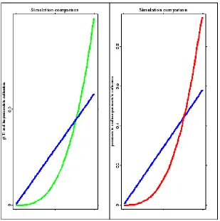
g0(t)(= t3_{) is based on (1.2.3). For comparison, we also calculate a parametric} fit for g0(t). Figure 2.1 shows the parametric estimate and nonparametric fitting forg0(t). The true curve is given by grey line(in the left side), the nonparametric estimate by thick curve(in the right side) and the parametric estimate by the black straight line.

Figure 2.1: Parametric and nonparametric estimates of the function g(T)

least squares estimates for the case where the variance is known up to a multiplicative constant. In his discussion, he assumed that the nonconstant vari-ance function ofY given (X, T) is an unknown smooth function of anexogenous

random vector W.

In the remainder of this section, we mainly consider model (1.1.1) with

heteroscedasticerror and focus on the following cases: (i)_{σ2

i}is an unknown

function of independentexogenousvariables; (ii)_{σ2

i}is an unknown function of

Ti; and (iii){σi2}is an unknown function ofXiTβ+g(Ti). We establish asymptotic

results for the three cases. In relation to our results, we mention recent devel-opments in linear and nonparametric regression models with heteroscedastic

errors. See for example,Bickel(1978),Box and Hill(1974),Carroll(1982),Carroll and Ruppert(1982),Carroll and H¨ardle (1989), Fuller and Rao(1978),Hall and Carroll(1989),Jobson and Fuller(1980),Mak(1992) andM¨uller and Stadtm¨uller

(1987).

Let _{(Yi, Xi, Ti), i= 1, . . . , n}denote a sequence of random samples from

Yi =XiTβ+g(Ti) +σiξi, i= 1, . . . , n, (2.1.3)

where (Xi, Ti) are i.i.d. random variables, ξi are i.i.d. with mean 0 and variance

1, andσ2

i are some functions of other variables. The concrete forms of σ2i will be

discussed in later subsections.

When the errors areheteroscedastic,βLS is modified to aweighted least

squaresestimator

βW =

_Xn

i=1

γiXfiXfiT

₋1_Xn

i=1

γiXfiYei

(2.1.4)

for some weightsγi i= 1, . . . , n. In this section, we assume that{γi} is either a

sequence of random variables or a sequence of constants. In our model (2.1.3) we take γi = 1/σi2.

In principle the weights γi (or σ2i) are unknown and must be estimated. Let

{γbi, i= 1, . . . , n} be a sequence of estimators of{γi}. We define an estimator of

β by substituting γi in (2.1.4) by γbi.

In order to develop the asymptotic theory conveniently, we use the tech-nique of split-sample. Let kn(≤ n/2) be the largest integer part of n/2. γbi(1)

. . . , (Xkn, Tkn, Ykn), and the later n−kn observations (Xkn+1, Tkn+1, Ykn+1), . . . ,

(Xn, Tn, Yn), respectively. Define

βW LS =

_Xn

i=1 b

γiXfiXfiT

₋1_Xkn

i=1 b

γ_i(2)XfiYei + n

X

i=kn+1

b

γ_i(1)XfiYei

(2.1.5)

as the estimator ofβ.

The next step is to prove thatβW LS is asymptotically normal. We first prove

thatβW is asymptotically normal, and then show that√n(βW LS−βW) converges

to zero in probability.

Assumption 2.1.1 sup_0≤t≤1E(_kX1k3|T =t)<∞. When {γi} is a sequence of

real numbers, then limn→∞1/nPni=1γiuiuTi = B, where B is a positive definite

matrix, and limn→∞1/nPni=1γi <∞. When {γi} is a sequence of i.i.d. random

variables, then B =E(γ1u1uT1) is a positive definite matrix.

Assumption 2.1.2 There exist constants C1 and C2 such that

0< C1 ≤min

i≤n γi ≤maxi≤n γi < C2 <∞.

We suppose that the estimator _{γbi} of {γi} satisfy

max

1≤i≤n|γbi−γi|=oP(n

−q_{) q}

≥1/4. (2.1.6)

We shall construct estimators to satisfy (2.1.6) for three kinds of γi later. The

following theorems present general results for the estimators of the parametric components in the partially linearheteroscedastic model (2.1.3).

Theorem 2.1.2 Assume that Assumptions 2.1.1, 2.1.2 and 1.3.2-1.3.3 hold. Then βW is an asymptotically normal estimator of β, i.e.,

√

n(βW −β)−→LN(0, B−1ΣB−1).

Theorem 2.1.3 Under Assumptions 2.1.1, 2.1.2 and (2.1.6), βW LS is

asymp-totically equivalent to βW, i.e., √n(βW LS −β) and √n(βW −β) have the same

Remark 2.1.1 In the case of constant error variance, i.e. σ2

i ≡ σ2, Theorem

2.1.2has been obtained by many authors. See, for example, Theorem 2.1.1.

Remark 2.1.2 Theorem2.1.3not only assures that our estimator given in (2.1.5) is asymptotically equivalent to the weighted LS estimator with known weights, but also generalizes the results obtained previously.

Before proving Theorems 2.1.2 and 2.1.3, we discuss three different variance functions and construct their corresponding estimates. Subsection 2.1.4 gives small sample simulation results. The proofs of Theorems 2.1.2 and 2.1.3 are postponed to Subsection 2.1.5.

2.1.2

Estimation of the Non-constant Variance Functions

2.1.2.1 Variance is a function of exogenous variables

This subsection is devoted to the nonparametric heteroscedasticity struc-ture

σ2_i =H(Wi),

where H is unknown and Lipschitz continuous, _{Wi;i = 1, . . . , n} is a

se-quence of i.i.d. design points defined on [0,1], which are assumed to be indepen-dent of (ξi, Xi, Ti).

Define

c

Hn(w) = n

X

j=1 e

ωnj(w){Yj−XjTβLS −bgn(Ti)}2

as the estimator of H(w), where _{ωenj(t);j = 1, . . . , n} is a sequence of weight

functions satisfying Assumption 1.3.3 with ωnj replaced byωenj.

Theorem 2.1.4 Assume that the conditions of Theorem 2.1.2 hold. Let cn =

n−1/3_{logn in Assumption 1.3.3. Then}

sup 1≤i≤n|

c

Proof. Note that c

Hn(Wi) = n

X

j=1 e

ωnj(Wi)(Yej −XfjTβLS)2

=

n

X

j=1 e

ωnj(Wi){XfjT(β−βLS) +ge(Ti) +εei}2

= (β₋βLS)T n

X

j=1 e

ωnj(Wi)XfjXfjT(β−βLS) + n

X

j=1 e

ωnj(Wi)eg2(Ti)

+

n

X

j=1 e

ωnj(Wi)eε2i + 2 n

X

j=1 e

ωnj(Wi)XfjT(β−βLS)eg(Ti)

+2

n

X

j=1 e

ωnj(Wi)XfjT(β−βLS)eεi+ 2 n

X

j=1 e

ωnj(Wi)eg(Ti)eεi. (2.1.7)

The first term of (2.1.7) is therefore OP(n−2/3) since Pnj=1XfjXfjT is a symmetric

matrix, 0<ωenj(Wi)≤Cn−2/3, n

X

j=1

{ωenj(Wi)−Cn−2/3}XfjXfjT

is a p_×p nonpositive matrix, and βLS −β = OP(n−1/2). The second term of

(2.1.7) is easily shown to be of order OP(n1/3c2n).

Now we need to prove sup i n X j=1 e

ωnj(Wi)eε2i −H(Wi)

=OP(n−1/3logn), (2.1.8)

which is equivalent to proving the following three results sup i n X j=1 e

ωnj(Wi)

n_Xn

k=1

ωnk(Tj)εk

o2

=OP(n−1/3logn), (2.1.9)

sup i n X j=1 e

ωnj(Wi)ε2i −H(Wi)

=OP(n−1/3logn), (2.1.10)

sup i n X j=1 e

ωnj(Wi)εj

n_Xn

k=1

ωnk(Tj)εko=OP(n−1/3logn). (2.1.11)

(A.3) below assures that (2.1.9) holds. Lipschitz continuity of H(_·) and as-sumptions onωenj(·) imply that

sup i n X j=1 e

ωnj(Wi)ε2i −H(Wi)

=OP(n−1/3logn). (2.1.12)

By taking aki = ωenk(Wi)H(Wk), Vk = ξ2k−1 r = 2, p1 = 2/3 and p2 = 0 in LemmaA.3, we have

sup i n X j=1 e

ωnj(Wi)H(Wj)(ξj2−1)

A combination of (2.1.13) and (2.1.12) implies (2.1.10). Cauchy-Schwarz inequal-ity, (2.1.9) and (2.1.10) imply (2.1.11), and then (2.1.8). The last three terms of (2.1.7) are all of order OP(n−1/3logn) by Cauchy-Schwarz inequality. We

therefore complete the proof of Theorem 2.1.4. 2.1.2.2 Variance is a function of the design points Ti

In this subsection we consider the case where _{σ2

i} is a function of {Ti}, i.e.,

σ_i2 =H(Ti), H unknown Lipschitz continuous.

Similar to Subsection 2.1.2.1, we define our estimator of H(_·) as

c

Hn(t) = n

X

j=1 e

ωnj(t){Yj −XjTβLS −gbn(Ti)}2.

Theorem 2.1.5 Under the conditions of Theorem 2.1.2, we have

sup 1≤i≤n|

c

Hn(Ti)−H(Ti)|=OP(n−1/3logn).

Proof. The proof of Theorem 2.1.5 is similar to that of Theorem 2.1.4 and therefore omitted.

2.1.2.3 Variance is a function of the mean Here we consider model (2.1.3) with

σ2

i =H{XiTβ+g(Ti)}, H unknown Lipschitz continuous.

This means that the variance is an unknown function of the mean response. Several related situations in linear and nonlinear models have been discussed by

Box and Hill(1974), Bickel(1978), Jobson and Fuller(1980),Carroll(1982) and

Carroll and Ruppert(1982).

Since H(_·) is assumed to be completely unknown, the standard method is to get information about H(_·) by replication, i.e., to consider the following “improved” partially linearheteroscedasticmodel

where_{Yij} is the response of the j−th replicate at the design point (Xi, Ti),ξij

are i.i.d. with mean 0 and variance 1,β,g(_·) and (Xi, Ti) are as defined in (2.1.3).

We here apply the idea of Fuller and Rao(1978) for linear heteroscedastic

model to construct an estimate of σ2

i. Based on the least squares estimate βLS

and the nonparametric estimategbn(Ti), we useYij − {XiTβLS +gbn(Ti)} to define

b

σ_i2 = 1

mi mi

X

j=1

[Yij − {XiTβLS +gbn(Ti)}]2, (2.1.14)

with a positive sequence_{mi; i= 1,· · ·, n}determined later.

Theorem 2.1.6 Let mi = ann2q

def

= m(n) for some sequence an converging to

infinity. Suppose the conditions of Theorem 2.1.2 hold. Then

sup 1≤i≤n|

b

σ_i2₋H_{X_iTβ+g(Ti)}|=oP(n−q) q≥1/4.

Proof. We provide only an outline for the proof of Theorem 2.1.6. Obviously

|σb_i2₋H_{X_iTβ+g(Ti)}| ≤3{XiT(β−βLS)}2 + 3{g(Ti)−gbn(Ti)}2

+ 3

mi mi

X

j=1

σ2_i(ξ_ij2 ₋1).

The first two items are obviouslyoP(n−q).Sinceξij are i.i.d. with mean zero and

variance 1, by takingmi =ann2q,using the law of the iterated logarithm and the

boundedness of H(_·), we have 1

mi mi

X

j=1

σ_i2(ξ_ij2 ₋1) =O_{m(n)−1/2logm(n)_}=oP(n−q).

Thus we derive the proof of Theorem 2.1.6.

2.1.3

Selection of Smoothing Parameters

In practice, an important problem is how to select the smoothing parameter involved in the weight functions ωni. Currently, the results on bandwidth

selec-tion for completely nonparametric regression can be found in the monographs by

Eubank (1988), H¨ardle (1990, 1991), Wand and Jones (1994), Fan and Gijbels

(1996), and Bowman and Azzalini (1997).

results for the case where the weight functions ωni are a sequence of orthogonal

series. See alsoGao(1998), who discussed the time series case and provided both theory and practical applications.

In this subsection, we briefly mention the selection procedure for bandwidth for the case where the weight function is a kernel weight.

For 1 _≤i_≤n, define e

ωi,n(t) = K

_t−Ti

h

. _Xn

j=1,j6=i

Kt−Tj h

,

e

gi,n(t, β) = n

X

j=1,j6=i

e

ωj,n(t)(Yj−XjTβ).

We now define the modified LS estimator βe(h) ofβ by minimizing

n

X

i=1

{Yi−XiTβ−gei,n(Ti, β)}2.

The Cross-Validation (CV) function can be defined as

CV(h) = 1

n

n

X

i=1

{Yi−XiTβe(h)−gei,n(Ti,βe(h))}2.

Letbhdenote the estimator ofh, which is obtained by minimizing the CV function CV(h) overh_∈Θh, where Θh is an interval defined by

Θh = [λ1n−1/5−η1, λ2n−1/5+η1],

where 0 < λ1 < λ2 <∞ and 0< η1 <1/20 are constants. Under Assumptions 1.3.1-1.3.3, we can show that the CV function provides an optimum bandwidth for estimating both β and g. Details for the i.i.d. case are similar to those in Section6.4.

2.1.4

Simulation Comparisons

We present a small simulation study to illustrate the properties of the theoretical results in this chapter. We consider the following model with different variance functions.

Yi =XiTβ+g(Ti) +σiεi, i= 1, . . . , n= 300,

where_{εi}is a sequence of the standard normal random variables,{Xi}and{Ti}

are mutually independent uniform random variables on [0,1], β = (1,0.75)T _and

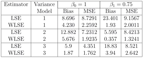
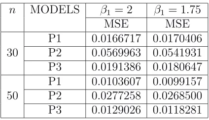
Table 2.1: Simulation results (_×10−3₎

Estimator Variance β0 = 1 β1 = 0.75 Model Bias MSE Bias MSE LSE 1 8.696 8.7291 23.401 9.1567 WLSE 1 4.230 2.2592 1.93 2.0011 LSE 2 12.882 7.2312 5.595 8.4213 WLSE 2 5.676 1.9235 0.357 1.3241 LSE 3 5.9 4.351 18.83 8.521 WLSE 3 1.87 1.762 3.94 2.642

Three models for the variance functions are considered. LSE and WLSE rep-resent the least squares estimator and the weighted least squares estimator given in (1.1.1) and (2.1.5), respectively.

• Model 1: σ2

i =Ti2;

• Model 2: σ2

i = Wi3; where Wi are i.i.d. uniformly distributed random

variables.

• Model 3: σ2

i = a1exp[a2{XiTβ +g(Ti)}2], where (a1, a2) = (1/4,1/3200). The case where g _≡0 has been studied by Carroll(1982).

From Table 2.1, one can find that our estimator (WLSE) is better than LSE in the sense of both bias and MSE for each of the models.

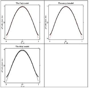
By the way, we also study the behavior of the estimate for the nonparametric part g(t)

n

X

i=1

ω∗_ni(t)(Yei −XfiTβW LS),

where ω∗

ni(·) are weight functions satisfying Assumption 1.3.3. In simulation,

we take Nadaraya-Watson weight function with quartic kernel(15/16)(1 ₋

2.1.5

Technical Details

We introduce the following notation, b

An = n

X

i=1 b

γiXfiXfiT, An = n

X

i=1

γiXfiXfiT.

Proof of Theorem 2.1.2. It follows from the definition ofβW that

βW −β =A−n1

n_Xn

i=1

γiXfige(Ti) + n

X

i=1

γiXfiεei

o

.

We will complete the proof by proving the following three facts for j = 1, . . . , p,

(i) H1j = 1/√nPni=1γixeijge(Ti) = oP(1);

(ii) H2j = 1/√nPni=1γixeijnPnk=1ωnk(Ti)ξk

o

=oP(1);

(iii) H3 = 1/√nPni=1γiXfiξi −→L N(0, B−1ΣB−1).

The proof of (i) is mainly based on Lemmas A.1 and A.3. Observe that

√

nH1j = n

X

i=1

γiuijgei+ n

X

i=1

γihnijgei− n X i=1 γi n X q=1

ωnq(Ti)uqjgei, (2.1.15)

wherehnij =hj(Ti)−Pnk=1ωnk(Ti)hj(Tk). In LemmaA.3, we taker = 2, Vk =ukl,

aji =gej, 1/4< p1 <1/3 and p2 = 1−p1. Then, the first term of (2.1.15) is

OP(n−(2p1−1)/2) =oP(n1/2).

The second term of (2.1.15) can be easily shown to be order OP(nc2n) by using

LemmaA.1.

The proof of the third term of (2.1.15) follows from Lemmas A.1 and A.3, and n X i=1 n X q=1

γiωnq(Ti)uqjegi

≤ C2nmax

i≤n |gei|maxi≤n

n X q=1

ωnq(Ti)uqj

= O(n2/3cnlogn) =op(n1/2).

Thus we complete the proof of (i).

We now show (ii), i.e., √nH2j →0.Notice that

√

nH2j = n

X

i=1

γi

n_Xn

k=1 e

xkjωni(Tk)

o ξi = n X i=1 γi

n_Xn

k=1

ukjωni(Tk)

o

ξi+ n

X

i=1

γi

n_Xn

k=1

hnkjωni(Tk)

o ξi − n X i=1 γi

h_Xn

k=1 n_Xn

q=1

uqjωnq(Tk)

o

ωni(Tk)

i

The order of the first term of (2.1.16) is O(n−(2p1−1)/2_{logn) by letting r = 2,}

Vk=ξk, ali =Pnk=1ukjωni(Tk), 1/4< p1 <1/3 and p2 = 1−p1 in Lemma A.3. It follows from Lemma A.1 and (A.3) that the second term of (2.1.16) is bounded by n X i=1 γi

n_Xn

k=1

hnkjωni(Tk)

o

ξi

≤ nmax

k≤n

n X i=1

ωni(Tk)ξi

max

j,k≤n|hnkj|

= O(n2/3cnlogn) a.s. (2.1.17)

The same argument as that for (2.1.17) yields that the third term of (2.1.16) is bounded by n X k=1 n_Xn

i=1

γiωni(Tk)ξi

on_Xn

q=1

uqjωnq(Tk)o

≤ nmax

k≤n

n X i=1

ωni(Tk)ξi

×max

k≤n

k X q=1

uqjωnq(Tj)

= OP(n1/3log2n) = oP(n1/2). (2.1.18)

A combination (2.1.16)–(2.1.18) implies (ii).

Using the same procedure as in Lemma A.2, we deduce that lim n→∞ 1 n n X i=1

γiXfiTXfi =B. (2.1.19)

A central limit theorem shows that asn_{→ ∞}

1 √ n n X i=1

γiXfiξi −→L N(0,Σ).

We therefore show that as n_{→ ∞}

1 √ nA −1 n n X i=1

γiXfiξi −→L N(0, B−1ΣB−1).

This completes the proof of Theorem2.1.2.

Proof of Theorem 2.1.3. In order to complete the proof of Theorem2.1.3, we only need to prove

√

n(βW LS−βW) = oP(1).

First we state a fact, whose proof is immediately derived by (2.1.6) and (2.1.19), 1

n|abn(j, l)−an(j, l)|=oP(n

forj, l = 1, . . . , p, whereban(j, l) and an(j, l) are the (j, l)−th elements of Abn and

An, respectively. The fact (2.1.20) will be often used later.

It follows that

βW LS −βW =

1 2 n

A_n−1(An−Abn)Ab−n1 n

X

i=1

γiXfige(Ti)

+Ab−_n1

kn

X

i=1

(γi−γbi(2))Xfige(Ti) +Ab−n1(An−Abn)Ab−n1 n

X

i=1

γiXfiξei

+Ab−_n1

kn

X

i=1

(γi−γbi(2))Xfiξei+Ab−n1 n

X

i=kn+1

(γi−bγi(1))Xfige(Ti)

+Ab−_n1

n

X

i=kn+1

(γi−γbi(1))Xfiξei

o

. (2.1.21)

ByCauchy-Schwarz inequality, for anyj = 1, . . . , p, n X i=1

γixeijge(Ti)

≤C√nmax

i≤n |eg(Ti)|

_Xn

i=1 e

x2_ij1/2,

which isoP(n3/4) by LemmaA.1and (2.1.19). Thus each element of the first term

of (2.1.21) is oP(n−1/2) by using the fact that each element of An−1(An−Abn)Ab−n1

isoP(n−5/4). The similar argument demonstrates that each element of the second

and fifth terms is alsooP(n−1/2).

Similar to the proof of H2j = oP(1), and using the fact that H3 converges to the normal distribution, we conclude that the third term of (2.1.21) is also

oP(n−1/2). It suffices to show that the fourth and the last terms of (2.1.21)

are both oP(n−1/2). Since their proofs are the same, we only show that for

j = 1, . . . , p,

n b

A−_n1

kn

X

i=1

(γi−γbi(2))Xfiξei

o

j =oP(n

−1/2₎

or equivalently

kn

X

i=1

(γi−γbi(2))exijξei =oP(n1/2). (2.1.22)

Let _{δn} be a sequence of real numbers converging to zero but satisfying

δn > n−1/4. Then for anyµ >0 and j = 1, . . . , p,

Pn

kn

X

i=1

(γi − γbi(2))exijξiI(|γi−γbi(2)| ≥δn)

> µn1/2o

≤ Pnmax

i≤n |γi−γb

(2)

i | ≥δn

o

The last step is due to (2.1.6). Next we deal with the term

Pn

kn

X

i=1

(γi−γbi(2))exijξiI(|γi−bγi(2)| ≤δn)

> µn1/2o

usingChebyshev’s inequality. Sinceγb_i(2)are independent ofξifori= 1, . . . , kn,

we can easily derive

En

kn

X

i=1

(γi−bγi(2))exijξi

o2 =

kn

X

i=1

E_{(γi−γbi(2))exijξi}2.

This is why we use the split-sample technique to estimateγi byγbi(2) and γb

(1)

i .

In fact,

Pn

kn

X

i=1

(γi − γbi(2))xeijξiI(|γi−γbi(2)| ≤δn)

> µn1/2o

≤

Pkn

i=1E{(γi−γbi(2))I(|γi−γbi(2)| ≤δn)}2EkXfik2Eξ2i

nµ2

≤ Cknδ

2

n

nµ2 →0. (2.1.24)

Thus, by (2.1.23) and (2.1.24),

kn

X

i=1

(γi−γbi(2))exijξi =oP(n1/2).

Finally,

kn

X

i=1

(γi − γbi(2))exij

n_Xn

k=1

ωnk(Ti)ξko

≤ √n

kn

X

i=1 f

X_ij21/2 max

1≤i≤n|γi−γb

(2)

i |₁max

≤i≤n

n

X

k=1

ωnk(Ti)ξk

.

This is oP(n1/2) by using (2.1.20), (A.3), and (2.1.19). Therefore, we complete

the proof of Theorem 2.1.3.

2.2

Estimation with Censored Data

2.2.1

Introduction

We are here interested in the estimation ofβ in model (1.1.1) when the response

Yi are incompletely observed and right-censored by random variables Zi. That

is, we observe

where Zi are i.i.d., and Zi and Yi are mutually independent. We assume that

Yi and Zi have a common distribution F and an unknown distribution G,

re-spectively. In this section, we also assume that εi are i.i.d. and that (Xi, Ti) are

random designs and that (Zi, XiT) are independent random vectors and

indepen-dent of the sequence_{εi}. The main results are based on the paper ofLiang and

Zhou(1998).

When the Yi are observable, the estimator of β with the ordinary rate of

convergence are given in (1.2.2). In present situation, the least squares form of (1.2.2) cannot be used any more since Yi are not observed completely. It is

well-known that in linear and nonlinear censored regression models, consistent estimators are obtained by replacing incomplete observations with synthetic data. See, for example, Buckley and James (1979), Koul, Susarla and Ryzin

(1981), Lai and Ying (1991, 1992) andZhou(1992). In our context, these suggest that we use the following estimator

b

βn =

h_Xn

i=1

{Xi−bgx,h(Ti)}⊗2

i₋1Xn

i=1

{Xi−gbx,h(Ti)}{Yi∗−gby∗_,h(T_i)} (2.2.2)

for somesynthetic data Y∗

i , whereA⊗2 def= A×AT.

In this section, we analyze the estimate (2.2.2) and show that it is asymptot-ically normal for appropriatesynthetic data Yi∗.

2.2.2

Synthetic Data and Statement of the Main Results

We assume that G is known first. The unknown case is discussed in the second part. The third part states the main results.

2.2.2.1 When G is Known Define synthetic data

Yi(1) =φ1(Qi, G)δi+φ2(Qi, G)(1−δi), (2.2.3)

whereφ1 and φ2 are continuous functions which satisfy (i). _{1₋G(Y)_}φ1(Y, G) +R_−∞Y φ2(t, G)dG(t) =Y; (ii). φ1 and φ2 don’t depend on F.

Remark 2.2.1 Equation (2.2.3) plays an important role in our case. Note that

E(Yi(1)|Ti, Xi) =E(Yi|Ti, Xi) by (i), which implies that the regressors ofYi(1) and

Yi on (W, X) are the same. In addition, if Z =∞, or Yi are completely observed,

thenYi(1) =Yi by takingφ1(u, G) =u/{1−G(u)}andφ2 = 0. So oursynthetic

data are the same as the original ones.

Remark 2.2.2 We here list the variances of the synthetic data for the follow-ing three pairs (φ1, φ2). Their calculations are direct and we therefore omit the details.

• φ1(u, G) = u, φ2(u, G) =u+G(u)/G′_(u),

Var(Yi(1)) =Var(Y) +

Z _∞

0 (

G(u)

G′_(u)

)2

{1₋F(u)_}dG(u).

• φ1(u, G) = u/_{1₋G(u)_}, φ2 = 0,

Var(Yi(1)) =Var(Y) +

Z _∞

0

u2_G(u)

1₋G(u)dF(u).

• φ1(u, G) = φ2(u, G) =R_−∞u _{1₋G(s)_}−1_ds,

Var(Yi(1)) =Var(Y) + 2

Z _∞

0 {1−F(u)} Z u

0

G(s)

1₋G(s)dsdG(u).

These arguments indicate that each of the variances ofYi(1) is greater than that of

Yi, which is pretty reasonable since we have modified Yi. We cannot compare the

variances for different(φ1, φ2), which depends on the behavior ofG(u). Therefore, it is difficult to recommend the choice of (φ1, φ2) absolutely.

Equation (2.2.2) suggests that the generalized least squares estimator of β is

βn(1) = (fXTfX)−1(fXTfY(1)) (2.2.4)

whereYf(1) denotes (Ye1(1), . . . ,Yen(1)) with Yei(1) =Yi(1)−Pnj=1ωnj(Ti)Yj(1).

2.2.2.2 When G is Unknown

construct our estimators, we need to assume G(sup_(X,W)TF(X,W)) ≤ γ for some known 0< γ <1, whereTF(X,W) = inf{y;F(X,W)(y) = 1}andF(X,W)(y) =P{Y ≤

y_|X, W_}.Let 1/3< ν <1/2 andτn= sup{t: 1−F(t)≥n−(1−ν)}.Then a simple

modification of the Kaplan-Meier estimator is

G∆n(z) =

    

b

Gn(z), if Gbn(z)≤γ,

γ, if z _≤maxQi and Gbn(z)> γ,

i= 1, . . . , n

whereGbn(z) is the Kaplan-Meier estimator given by

b

Gn(z) = 1−

Y

Qi≤z

1₋ 1

n₋i+ 1 (1−δi)

.

Substituting G in (2.2.3) by G∆

n, we get thesynthetic data for the case of

unknown G(u), that is,

Yi(2) =φ1(Qi, G∆n)δi+φ2(Qi, G∆n)(1−δi).

Replacing Yi(1) in (2.2.4) by Yi(2), we get an estimate of β for the case of

un-known G(_·). For convenience, we make a modification of (2.2.4) by employing thesplit-sampletechnique as follows. Letkn(≤n/2) be the largest integer part

ofn/2. Let G∆

n1(•) and G∆n2(•) be the estimators of Gbased on the observations (Q1, . . . , Qkn) and (Qkn+1, . . . , Qn), respectively. Denote

Y_i(1)₍₂₎ =φ1(Qi, G∆n2)δi+φ2(Qi, G∆n2)(1−δi) for i= 1, . . . , kn

and

Y_i(2)₍₂₎ =φ1(Qi, G∆n1)δi+φ2(Qi, G∆n1)(1−δi) fori=kn+ 1, . . . , n.

Finally, we define

βn(2) = (fXTfX)−1 n_Xkn

i=1 f

X_i(1)Ye_i(1)₍₂₎+

n

X

i=kn+1

f

X_i(2)Ye_i(2)₍₂₎o

as the estimator ofβ and modify the estimator given in (2.2.4) as

βn(1) = (XfTfX)−1 n_Xkn

i=1 f

X_i(1)Ye_i(1)₍₁₎+

n

X

i=kn+1

f

where e

Y_i(1)₍₂₎ =Y_i(1)₍₂₎₋

kn

X

j=1

ωnj(Ti)Y_j(1)₍₂₎, Ye_i(2)₍₂₎ =Y_i(2)₍₂₎− n

X

j=kn+1

ωnj(Ti)Y_j(2)₍₂₎

e

Y_i(1)₍₁₎ =Yi(1)−

kn

X

j=1

ωnj(Ti)Yj(1), Yei(2)(1) =Yi(1)−

n

X

j=kn+1

ωnj(Ti)Yj(1)

f

Xi(1) =Xi− kn

X

j=1

ωnj(Ti)Xj, Xfi(2) =Xi− n

X

j=kn+1

ωnj(Ti)Xj.

2.2.2.3 Main Results

Theorem 2.2.1 Suppose that Assumptions 1.3.1-1.3.3 hold. Let (φ1, φ2) ∈ K and E_|X_|4 _{<∞. Then β}

n(1) is an asymptotically normal estimator of β, that is,

n1/2_(β

n(1)−β)−→L N(0,Σ∗) where Σ∗ _{= Σ}−2_E{ǫ2

1(1)u1uT1} with ǫ1(1)=Y1(1)−E{Y1(1)|X, W}. Let _K∗ _{be a subset of K, consisting of all the elements (φ}

1, φ2) satisfying the following: There exists a constant 0<_C <_∞such that

max

j=1,2,u≤s|φj(u, G)|<C for all s with G(s)<1

and there exist constants 0< L=L(s)<_∞ and η >0 such that

max

j=1,2,u≤s|φj(u, G

∗_)−φ

j(u, G)| ≤Lsup u≤s|G

∗_(u)−G(u)|

for all distribution functionsG∗ _{with sup}

u≤s|G∗(u)−G(u)| ≤η.

Assumption 2.2.1 Assume that F(w) and G(w) are continuous. Let Z TF

−∞

1

1₋F(s)dG(s)<∞.

Theorem 2.2.2 Under the conditions of Theorem 2.2.1 and Assumption 2.2.1,