A Genetic Algorithm based Fuzzy C Mean Clustering
Model for Segmenting Microarray Images
Biju V G
Division of Electronics School Of EngineeringCochin university of Science and Technology
Mythili P
Division of Electronics School Of EngineeringCochin university of Science and Technology
ABSTRACT
Genetic algorithm based Fuzzy C Mean (GAFCM) technique is used to segment spots of complimentary DNA (c-DNA) microarray images for finding gene expression is proposed in this paper. To evaluate the performance of the algorithm, simulated microarray slides were generated whose actual mean values were known and is used for testing. K-means, Fuzzy C Means (FCM) and the proposed GAFCM algorithm were applied to the simulated images for the separation of the foreground (FG) spot signal information from background (BG) and the results were compared. The strength of the algorithm was tested by evaluating the segmentation matching factor, coefficient of determination, concordance correlation and gene expression values. From the results it is observed that the segmentation ability of GAFCM is better compared to FCM and K- Means algorithms.
Keywords
K-means, FCM, GAFCM, Genetic Algorithm, Segmentation, Gene expression
1.
INTRODUCTION
C-DNA microarrays is one of the most fundamental and powerful tools in biotechnology, which has been utilized in many biomedical applications such as cancer research, infectious disease diagnosis and treatment, toxicology research, pharmacology research, and agricultural development. The enormous improvement of technology in the last decade provides the ability to simultaneously identify and quantify thousands of genes by their gene expression [1]. The spots on a microarray are segmented from the background to compute the red to green intensity ratio to give the gene expression. The three basic operations to compute the spot intensities are gridding, segmentation and intensity extraction. These operations are used to find the accurate location of the spot, separate spot FG from BG and the calculation of the mean red and green intensity ratio. In the last decade, several software packages and algorithms were developed for segmenting spots in microarray images. Fixed circle segmentation was the first algorithm used in ScanAlyze Software [2], where all spots were considered to be circular with a predefined fixed radius. An adaptive circle segmentation technique was employed in the GenePix software [3], where the radius of each spot was not considered constant but adapts to each spot separately. Dapple software estimated the radius of the spot using the laplacian based edge
detection [4]. An adaptive shape segmentation technique was used in the Spot software [5]. A histogram-based segmentation method was used in the ImaGene software [6]. Later watershed [7] and the seeded region algorithms [8] were employed. The disadvantage of the above mentioned software packages and algorithms were either the spots were considered to be circular in shape or a priori knowledge of the precise position of the spot’s center was a prerequisite [9]. Further segmentation algorithms based on the statistical Mann–Whitney test were also used [10], which assess the statistical significant difference between the FG and BG. Lately the K-Means and FCM clustering algorithm are the techniques that are used for spot segmentation [11][12]. The present work mainly focuses on the microarray spot segmentation ability of the proposed GAFCM algorithm over the FCM and K-mean algorithm. Gridding is done by means of an automatic gridding based on intensity profile technique using both horizontal and vertical intensity profiles and the spots are addressed on the basis of this gridding information. The K-means, FCM and GAFCM algorithm were developed in matlab [13]. For the evaluation and testing of the algorithm both simulated and real microarray images were used. The performance of the algorithms were tested by evaluating the segmentation matching factor (SMF), Coefficient of determination (r2),Concordance correlation (Pc)
and spot gene expression value.
2.
METHODS
[15] is given in Section 3 and the proposed GAFCM is described in detail in Section 4.
Figure 1 Block diagram of microarray image processing.
3.
FUZZY
C
MEAN
(FCM)
ALGORITHM
Let x= xi, i = 1 to N be the pixels of a single microarray spot,
where N is the number of pixels present in the spot. These pixels have to be clustered in two classes BG and FG. Let cj
j=1,2 be the cluster centers of the FG and BG pixels respectively. Each pixel should have membership degrees uij
for each cluster. The pixel is assigned to a particular cluster based on the value of the membership degree function. Hence the algorithm aims at iteratively improving the membership degree function until there is no change in the cluster centers.
The sum of the membership values of a pixel belonging to all clusters should satisfy Equation 1.
∑
(1)
The Euclidean distance from a pixel to a cluster center is given by
(2)
The aim of this method is to minimize the absolute value of the difference between the two consecutive objective functions Ft and Ft+1 given by the Equation 3 and 4.
∑
∑
(3)
(4)
Where m is the fuzziness parameter and ε is the error which has to be minimized. Iteratively in each step, the updated membership uij and the cluster centers cj are given by Equations 5 and 6. ∑
(5)
∑
(6)
4. GENETIC ALGORITHM BASED FCM
OPTIMIZATION (GAFCM).
GA is a powerful, stochastic non-linear optimization tool based on the principles of natural selection and evolution [16][17][18][19][20]. To find the optimum fuzzy partitions of a microarray spot signal, a new GA based fuzzy c mean clustering method has been proposed. Clustering using GAFCM can be achieved using the following steps. Here each chromosome in the population of GA encodes a possible partition of image and the goodness of the chromosome is computed by using a fitness function. The technique is described as follows.A.
Population initialization
The chromosomes are made up of real numbers which represent microarray spot BG and FG pixel intensity centers respectively. These values are randomly initialized by taking all possible intensity values in the search space under evaluation.B.
Fitness computation
Fitness of a chromosome is calculated in two steps. In the first step membership values of the image data points to the different clusters are computed by using FCM algorithm. In the second step fitness value is computed. This is used as a measure to evaluate the fitness of the chromosome. The membership degree function uij can be computed using the FCM algorithm explained in Section 3. Saha et.al has given a fitness function for the segmentation of satellite images [21][22]. This has been further modified for finding the cluster center of c-DNA microarray spots and is given in Equation 7.(7)
Where
(8)
(9)
(10)
Ec is same as Equation 4. This is the difference between
two successive objective function values in FCM. This value is to be minimized. Dc is the maximum Euclidean
distance between two cluster centers among all centers. E is the error matrix; Gijis a 2x N reference matrix. The first row of the reference matrix is the one dimensional binary image corresponding to the simulated spot. The second row is the complement of first row. The objective is to maximize the Fit so as to achieve proper clustering. To ensure this E & Ec values has to decrease and Dc has
DNA Microarray
image
Gridding
Automatic spot cropping based on
gridding
Segmentation of spot from
background Red and
Green channel intensity extraction Computation
C.
Selection, Crossover and Mutation
Roulette wheel selection method is applied on the population where, each chromosome receives a number that is proportional to its fitness value. Crossover and Mutation are the two Genetic Operators used for the creation of new Chromosomes. After repeating steps A, B, C for a fixed number of iterations the best cluster centers are selected [23]. The flow chart for performing GAFCM is given in Figure 2
No
Yes
Figure 2 Flow chart of GAFCM algorithm.
5. EVALUATION OF THE PROPOSED
METHOD
To quantify the effectiveness of the proposed approach, simulated as well as real microarray images from the Stanford Microarray Database (SMD) have been used. The spots were gridded and segmented using K-Means, FCM and GAFCM independently for comparison purposes. Simulated microarray images were used for validation and comparison purposes since their gene expressions are known. Spots were simulated with realistic characteristics to ensure that it looks like a true c-DNA image, consisting of more than 1000 spots. Hence a real c-DNA image was used as a template, and its binary version was produced by employing a threshold technique [24]
After converting it into a binary image, the spot area is replaced by random values of mean intensities. In the simulated microarray image the mean intensity value of each spot was predefined, ranging between 0 and 255 for both the R and G channels [24]. BG intensities were replaced by a single intensity value.
The accuracy of any segmentation technique can be evaluated using three parameters. The segmentation matching factor SMF, The coefficient of determination r2 and The concordance correlation Pc. The SMF [25][26][27] for every
binary spot, produced by the clustering algorithm is given by
(11)
Where Aseg is the area of the spot, as determined by the
proposed algorithm and Aact is the actual spot area. A perfect
match is indicated by a 100% score, any score higher than 50% indicates reasonable segmentation where as a score less than 50% indicate poor segmentation. The coefficient of determination r2 [24][28][29] indicates the strength of the linear association between simulated and calculated spots, as well as the proportion of the variance of the calculated data.
∑∑
(12)
Where Iseg and Iact are the mean intensity value of the
calculated and simulated spots respectively and Imean is the
overall mean spot intensity values of the simulated image. The algorithm that scores r2 value closer to 1 has better performance.
The concordance correlation Pc was calculated using the Equation
̅ ̅
(13)
StartCrop the spot sub image based on Gridding
Initialize the center encoded population matrix P (K) of size (Nx2)
Select chromosome
Update uij matrix
matrix
Calculate cj matrix based on uij
Find Ec, E, Dc and Fit matrix
Selection, Cross over & Mutation
Update the population matrix P (K)
If (iterations= desired value)
Select the best uij, cj & Cluster the spot
pixels into BG & FG
Stop
A
Where A and B are two samples, ̅ ̅ are the mean values, and SA and SB are the standard deviation of the samples. The
higher the Pc value, the better the performance of the
algorithm. Further the proposed algorithm’s performance has been tested in the presence of noise. This was done by corrupting the simulated spot with additive white Gaussian noise whose signal-to-noise ratio (SNR) ranges from 1 to 19 dB [30].
6.
RESULTS AND DISSCUSSION
The segmentation ability of KM, FCM and the proposed GAFCM algorithm is made by computing and comparing the SMF r2 and Pc values explained in section 5. The K-Means,
FCM and GAFCM algorithms were applied independently on these images for the classification of the BG and FG pixels. Several microarray images with different FG mean were simulated and spots were randomly selected from these images. The SMF value for the three algorithms is shown in Figure 3 with the original spots, actual boundaries and the results obtained for various methods. It is obvious from the result that GAFCM shows an overall SMF of 98.56% compared to FCM with 97.19% and K-means with 68.78%. The average SMF, r2 and Pc values shown in Table 1 is
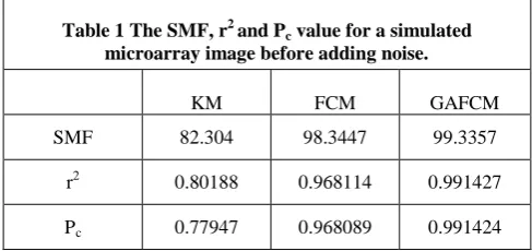
[image:4.595.317.522.322.646.2]obtained from the simulated microarray image shown in Figure 4 before corrupting it with noise.
Table 1 The SMF, r2 and P
c value for a simulated
microarray image before adding noise.
KM FCM GAFCM
SMF 82.304 98.3447 99.3357
r2 0.80188 0.968114 0.991427
Pc 0.77947 0.968089 0.991424
The segmentation ability of the proposed method in the presence of noise has been studied. To do this, the simulated microarray images were added with additive white Gaussian noise gradually. The SMF, r2 and Pc values of the noisy
images were computed using K-means, FCM and GAFCM algorithm. The SNR value is varied from 1dB to 19 dB. Figure 5 shows the graph of SMF vs SNR for the three algorithms and Table 2 gives the corresponding numerical value. It can be seen from the graph that the difference in the SMF is more for FCM and GAFCM compared with K- means. In the case of GAFCM and FCM even though curves are close, GAFCM segmentationis better than FCM for low and high noise images. The result showsthat the overall SMF value varies from 97.050% to70.551%, 96.807% to 69.645% and 85.418% to 53.940% for GAFCM, FCM and K-means respectively. This reveals that GAFCM is having better SMF value.
The Coefficient of determination (r2) for simulated microarray images for K-means, FCM and GAFCM are shown in Table 3. The graph between r2 and SNR in dB is shown in Figure 6. The method that scores r2 value closer to 1 has better performance. The r2 value of GAFCM is closer to 1 compared to FCM and K-means for low noise images. The variation of r2 for SNR variation from 1 to 19 dB is from 0.7501 to 0.1296, 0.6935 to 0.1079 and 0.2880 to 0.0036 for GAFCM, FCM and K-means respectively.
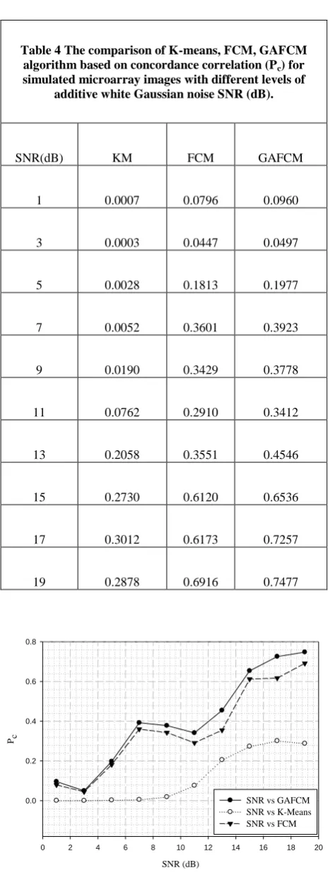
The concordance correlation (Pc) values obtained for
K-means, FCM and GAFCM are shown in Table 4. Figure 7 shows the graph between Pc and SNR in dB. Higher the values
of Pc the better will be the segmentation value for that
algorithm. From Table 4 it can be seen that the Pc value varies
from 0.7471 to 0.0960, 0.6916 to 0.0796 and 0.2878 to 0.0007 for GAFCM, FCM and K-mean respectively. This clearly indicates that the proposed GAFCM has better segmentation capability for the current application.
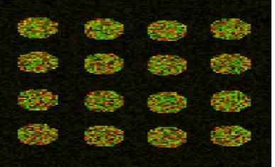
[image:4.595.51.295.397.512.2]
Figure 4 Simulated microarray image used to calculate the gene expression.
SNR(dB)
0 2 4 6 8 10 12 14 16 18 20
SMF
50 60 70 80 90 100
SNR vs GAFCM SNR vs K-Means SNR vs FCM
Figure 5 SMF calculated for simulated image corrupted with additive white Gaussian noise having different levels
[image:5.595.72.266.72.190.2]of SNR (dB) using K-means, FCM, GAFCM algorithms.
Table 2 The comparison of K-means, FCM, GAFCM algorithm based on segmentation matching factor
(SMF) for simulated microarray images with different levels of additive white Gaussian noise
SNR(dB).
SNR(dB) KM FCM GAFCM
1 53.93972 69.64504 70.55050
3 58.52296 78.66445 79.11223
5 63.03961 84.53164 84.63773
7 67.87467 88.79217 89.11575
9 72.60327 92.44617 92.73175
11 77.90749 92.61146 93.02225
13 81.82369 94.17475 94.70089
15 84.01279 95.58631 96.18429
17 85.22194 96.1873 96.28328
19 85.41774 96.80675 97.05008
Table 3 The comparison of K-means, FCM, GAFCM algorithm based on coefficient of determination (r2) for simulated microarray images
with different levels of additive white Gaussian noise SNR(dB).
SNR(dB) KM FCM GAFCM
1 0.003582 0.107935 0.129569
3 0.002433 0.070657 0.08278
5 0.009682 0.200522 0.217191
7 0.014513 0.380952 0.414809
9 0.034473 0.348032 0.382025
11 0.091063 0.310028 0.361558
13 0.211104 0.35561 0.454974
15 0.273211 0.613217 0.657108
17 0.301239 0.619506 0.728683
19 0.287993 0.693543 0.750119
SNR (dB)
0 2 4 6 8 10 12 14 16 18 20
r
2
0.0 0.2 0.4 0.6 0.8
SNR vs GAFCM SNR vs K-Means SNR vs FCM
Figure 6 r2 calculated for simulated image corrupted with additive white Gaussian noise having different levels of
[image:5.595.54.272.238.392.2] [image:5.595.51.277.455.763.2]Table 4 The comparison of K-means, FCM, GAFCM algorithm based on concordance correlation (Pc) for
simulated microarray images with different levels of additive white Gaussian noise SNR (dB).
SNR(dB) KM FCM GAFCM
1 0.0007 0.0796 0.0960
3 0.0003 0.0447 0.0497
5 0.0028 0.1813 0.1977
7 0.0052 0.3601 0.3923
9 0.0190 0.3429 0.3778
11 0.0762 0.2910 0.3412
13 0.2058 0.3551 0.4546
15 0.2730 0.6120 0.6536
17 0.3012 0.6173 0.7257
19 0.2878 0.6916 0.7477
SNR (dB)
0 2 4 6 8 10 12 14 16 18 20
Pc
0.0 0.2 0.4 0.6 0.8
SNR vs GAFCM SNR vs K-Means SNR vs FCM
Figure 7 Pc calculated for simulated image corrupted with
additive white Gaussian noise having different levels of SNR (dB) using K-means, FCM, GAFCM algorithms.
[image:6.595.315.564.294.609.2]The aim of microarray image processing is to find the gene expression value. The gene expression value is the logarithm mean intensity ratio of red and green channels in a spot. The closeness of the computed gene expression value with the actual value shows the performance of the algorithm. To validate this, several microarray images were simulated and tested. Figure 4 shows one such simulated images and the corresponding result is shown in Table 5. The better the segmentation technique the closer will be the gene expression value with the actual value. Table 5 shows the gene expression value obtained for a microarray simulated image of 16 spots using the three segmentation methods along with their actual values of gene expression.It can be seen that the gene expression value measured is almost close to the actual value in the case of GAFCM compared to FCM and K-Means. This shows that GAFCM algorithm has better scope in microarray image spot segmentation application.
Table 5 Comparison of gene expression values computed using K-means, FCM and GAFCM algorithm.
SPOT No
Gene Expression
KM FCM GAFCM Actual
1 -0.01147 -0.06477 -0.04779 -0.04779 2 0.04617 -0.12034 -0.12034 -0.12034 3 0.03171 -0.09431 -0.09431 -0.09431 4 0.16624 0.08583 0.085828 0.091598 5 -0.12983 -0.19036 -0.17852 -0.17852 6 -0.00411 -0.11734 -0.11734 -0.10333 7 -0.05711 -0.1459 -0.13697 -0.13276 8 0.12509 -0.00511 -0.00511 -0.00386 9 -0.02495 -0.07131 -0.07716 -0.07716 10 -0.04111 -0.09078 -0.09078 -0.09078 11 -0.05853 -0.15023 -0.15023 -0.15023 12 0.06195 0.0167 0.016696 0.016696 13 -0.02509 -0.10586 -0.09059 -0.09059 14 0.03494 -0.04701 -0.04701 -0.04922 15 -0.11408 -0.2259 -0.2259 -0.2259 16 0.0467 -0.07544 -0.0705 -0.02818
7. CONCLUSION
levels. This can be rectified by using suitable filtering techniques. As our future work, the noise removal has to be addressed to get much smoother image and also an improved clustering algorithm is to be developed so that low signal intensity spots can be segmented more effectively.
8. REFERENCES
[1] Y. H. Yang, M. J. Buckley, S. Duboit, and T. P. Speed (2002), “Comparison of methods for image analysis on c- DNA microarray data,” J. Comput. Graphical Statist., vol. 11, pp. 108–136
[2] M.B.Eisen. (1999). ScanAlyze [Online] http://rana.lbl.gov/ EisenSoftware.htm
[3] GenPix 4000, A User’s Guide (1999), Axon Instruments, Inc., Foster City, CA.
[4] J. Buhler, T. Ideker, and D. Haynor, “Dapple: improved techniques for finding spots on DNA microarrays,” Technical Report. UWTR 2000-08-05, UV CSE, Seattle,Washington, USA.
[5] M. J. Buckley. (2000). The spot user’s guide. CSIRO Mathematical and Information Science [Online].
Available:
http://www.cmis.csiro.au/IAP/Spot/spotmanual.html.
[6] ImaGene, ImaGene 6.1 User Manual. (2006. [Online]
Available:-http://www.biodiscovery.com/index/papps-webfiles-action.
[7] S. Beucher and F. Meyer (1993), “The morphological approach to segmentation: The watershed transformation,” Opt. Eng., vol. 34, pp. 433–481. [8] R. Adams and L. Bischof (Jun. 1994), “Seeded region
growing,” IEEE Trans. Pattern Anal. Mach. Intell., vol. 16, no. 6, pp. 641–647.
[9] D. Bozinov and J. Rahenfuhrer (2002.), “Unsupervised technique for robust target separation and analysis of DNA microarray spots through adaptive pixel clustering,” J. Bioinform., vol. 18, pp. 747–756. [10] Y. Chen, E. R. Dougherty, and M. L. Bittne (1997),
“Ratio-based decisions abd the quantitative analysis of c-DNA microarray images,” J. Biomed. Opt., vol. 2, pp. 264–374.
[11] S. Wu and H. Yan (2003), “Microarray Image Processing Based on Clustering and Morphological Analysis”, Proc. Of First Asia-Pasific Bioinformatics Conference, Adelaide, Australia, pp. 111-118.
[12] Volkan Uslan and Đhsan Ömür Bucak (2010). Microarray image segmentation using clustering methods. Mathematical and Computational Applications, Vol. 15, No. 2, pp. 240-247, © Association for Scientific Research
[13] The Math Works, Inc., Software, MATLABR (2010a). Natick, MA.
[14] MacQueen, J. B. (1967). Some Methods for classifications. In 5-th Berkeley Symposium on Mathematical Statistics and Probability, 1, 281-297. Berkeley:University of California Press
[15] J. C. Bezdek (1981), Pattern Recognition with Fuzzy Objective Function Algorithms, Plenum Press, New York.
[16] D. E. Goldberg (1989), Genetic Algorithms in Search, Optimization & Machine Learning, Boston: Addison-Wesley, Reading, ch. 1.
[17] L.Davis (Ed.)(1991), Handbook of Genetic Algorithms, Van Nostrand Reinhold, New York.
[18] Z. Michalewicz (1992), Genetic Algorithms #Data Structures" Evolution Programs, Springer, New York. [19] J.L.R. Filho, P.C. Treleaven, C. Alippi (1994), Genetic
algorithm programming environments, IEEE Comput. 27, 28-43.
[20] U. Maulik and S. Bandyopadhyay (2000), “Genetic algorithm based clustering technique,” Pattern Recog., vol. 33, pp. 1455–1465.
[21] Saha, S. and Bandyopadhyay, S., Accepted, (2007), Fuzzy Symmetry Based Real-Coded Genetic Clustering Technique for Automatic Pixel Classification in Remote Sensing Imagery. Fundamenta Informaticae.
[22] S. Bandyopadhyay and S. Saha (2007), “GAPS: A clustering method using a new point symmetry based distance measure,” Pattern Recog., vol. 40, pp. 3430– 3451.
[23] F. Herrera, M. Lozano, and J. L. Verdegay (Nov 1998), “Tackling Real Coded Genetic Algorithms: Operators and Tools for Behavioural Analysis,” Artificial Intelligence Review, vol. 12, no. 4, pp. 265–319. [24] O. Demirkaya, M. H. Asyali, and M.M. Shoukri (2005),
“Segmentation of c-DNA microarray spots using Markov radom field modeling,” Bioinformatics, vol. 21, no. 13, pp. 2994–3000.
[25] D. Tran and M. Wagner (2002), “Fuzzy C-means clustering-based speaker verification,” in Lecture Notes in Computer Science: Advances in Soft Computing— AFSS 2002, N. R. Pal and M. Sugeno, Eds. New York: Springer-Verlag, pp. 318–324.
[26] D. Betal, N. Roberts, and G. H. Whitehouse (1997), “Segmentation and numerical analysis of micro calcifications on mammograms using mathematical morphology,” Br. J. Radiol., vol. 70, no. 837, pp. 903– 917.
[27] E.I. Athanasiadis, D.A. Cavouras, P.P. Spyridonos, D.Th.Glotsos, I.K. Kalatzis, G.C. Nikiforidis (July 2009), Complementary DNA microarray image processing based on the Fuzzy Gaussian mixture model, in: IEEE Transaction on Information Technology in Biomedicine, vol. 13, issue 4.
[28] E.I. Athanasiadis, D.A. Cavouras, P.P. Spyridonos, D.Th.Glotsos, I.K. Kalatzis, G.C. Nikiforidis (2011), A Wavelet based markov random field segmentation model in segmenting microarray experiments, in: Computer methods and programs in biomedicine 104,307-315. [29] A.Lehmussola, et al. (2006), Evaluating the performance
of microarray segmentation algorithms, Bioinformatics 22, 2910–2917.