http://dx.doi.org/10.4236/wsn.2015.77008
How to cite this paper: Sheu, T.-L., Kuo, Y.-H. and Chou, Z.-T. (2015) A Packet-Interleaving Scheme Using RS Code for Burst Errors in Wireless Sensor Networks. Wireless Sensor Network, 7, 83-99. http://dx.doi.org/10.4236/wsn.2015.77008
A Packet-Interleaving Scheme Using RS Code
for Burst Errors in Wireless Sensor
Networks
Tsang-Ling Sheu, Yen-Hsi Kuo, Zi-Tsan Chou*
Department of Electrical Engineering, National Sun Yat-Sen University, Kaohsiung Taiwan Email: [email protected], [email protected], *[email protected]
Received 27 May 2015; accepted 10 July 2015; published 13 July 2015
Copyright © 2015 by authors and Scientific Research Publishing Inc.
This work is licensed under the Creative Commons Attribution International License (CC BY).
http://creativecommons.org/licenses/by/4.0/
Abstract
In this paper, we propose a packet-interleaving scheme (PIS) for increasing packet reliability un-der burst errors in wireless sensor networks (WSN). In a WSN, packet errors could occur due to weak signal strength or interference. These erroneous packets have to be retransmitted, which will increase network load substantially. The proposed PIS, encoding data using Reed-Solomon (RS) codes, can classify data into two different types: high-reliability-required (HRR) data and non-HRR data. An HRR packet is encoded with a short RS symbol, while a non-HRR packet with a long RS symbol. When an HRR and a non-HRR packet arrive at a sensor, they are interleaved on a symbol-by-symbol basis. Thus, the effect of burst errors (BE) is dispersed and consequently the uncorrectable HRR packets can be reduced. For the purpose of evaluation, two models, the uni-form bit-error model (UBEM) and the on-off bit-error model (OBEM), are built to analyze the packet uncorrectable probability. In the evaluation, we first change the lengths of BE, then we vary the shift positions in a BE period, and finally we increase the number of correctable symbols to observe the superiority of the proposed PIS in reducing packet uncorrectable probability.
Keywords
WSN, RS Code, Burst Errors, Interleaving, Packet Uncorrectable Probability
1. Introduction
Along with the increasing requirements for living quality and home security, sensors have been widely deployed inside or outside a building to collect environmental information, such as temperature, humidity, image, motion
picture, etc. To effectively deliver the collected data back to a control center for further analysis, a wireless sen-sor network (WSN) [1]-[3] is usually built. However, packet transmission over a WSN may encounter intermit-tent errors due to weak signals or interferences. The erroneous packets, if comprising of text or numbers, such as temperature or humidity, would require packet re-transmission, which surprisingly increases network load. Thus, the motivation of this paper is to increase transmission reliability over a WSN, which has recently attracted many researchers’ attention.
Basically, previous researches on transmission reliability over a WSN can be divided into three major catego-ries: reliable routing, information coding, and network coding. In the first category, to increase the transmission reliability after data are collected by a sensor node, relay nodes (RNs) are employed. For examples, H. Chebbo,
et al.[4] modified IEEE 802.15.4 MAC frames. The authors added one bit in the frame control field, with which whether it is necessary to build a tree by RNs or just build a simple star, can be determined. Moreover, R. Sam-pangi, et al.[5] utilized RNs to divide sensors into several cluster networks. Since the distance from a sensor to its cluster head is reduced, the quality of data transmission is greatly improved. To protect the routing path, S. Kim, et al. [6] utilized both coding and retransmission schemes once the established path fails. However, in these schemes, it is inevitable that end-to-end packet delay will increase accordingly due to multiple-hop for-warding.
Thus, in the second category, instead of developing reliable routing, the authors switch their interests to in-formation coding. For examples, E. Byrne, et al.[7] designed a coding scheme which can increase the probabil-ity of successful decoding based on graph theory. Y. Hamada, et al.[8] proposed a scheme to reduce packet er-ror rate by using Luby Transform (LT) codes [9]. Their proposed schemes have achieved small complexity of O(n); yet too many packets are required for retransmission when bit error rate is high. Thus, K. Ishibashi, et al.
[10] proposed embedded forward error control (FEC) technique which utilizes RS (Reed Solomon) code to
re-duce packet error rate. Similarly, M. Busse, et al.[11] can recover lost chunk by using Fountain code and Raptor code. To increase data reliability and processing speed, K. Yu, et al. [12] designed new FEC which protects header and payload, respectively. Similarly, M. Srouji, et al.[13] proposed a reliable data transfer scheme which can adjust the lengths of redundancy code based on the successful receiving rate at the downstream node.
In the third category, to increase transmission reliability, researchers focus on network coding. For examples, to increase the probability of successfully recovering the transmitted data, G. Arrobo, et al.[14] proposed coop-erative network coding. Similarly, A. Taparugssanagorn, et al. [15] proposed unequally error protection (UEP) scheme. In UEP, data are classified into two types: medical and non-medical. Only medical data are EX-ORed, while non-medical data are not. However, in UEP, it is not guaranteed that a downstream sensor node can al-ways decode data successfully. Thus, I. Salhi, et al.[16] proposed another reliable coding scheme where a relay node can produce much better packet combination through the exchange of neighboring table and topology in-terference information. Finally, Z. Kiss, et al.[17] tried to combine two coding techniques, RS coding and net-work coding. Once a relay node receives data packets transmitted from all the downstream sensor nodes, it be-gins to chop every data packet into smaller segments. Each segment is encoded into two symbols using RS codes. The two symbols are then converted to two checking blocks before data transmission. A receiving node can therefore increase the probability of correct data by decoding these two checking blocks.
Unlike the previous research work, where the authors focused on reliable routing, information coding, and network coding, in this paper, we propose a packet interleaving scheme (PIS) to reduce the impact of burst er-rors (BE) on high-reliability-required (HRR) data in WSNs. BE is defined as a sequence of transmitted bits which may encounter errors in continuous bit pattern. Although Reed-Solomon (RS) codes [18], which encode data in a block-by-block fashion, may correct bit errors in a certain constraints, it may not be economically wor-thy in dealing with burst errors when the number of consecutive bit errors exceeds a threshold. In other words, it makes the overhead of redundancy codes become unacceptable. Hence, to increase packet correctable probabil-ity in a WSN, the proposed PIS first classifies the collected data into two different types: HRR data and non-HRR data. An HRR packet is encoded with a short RS symbol, while a non-HRR packet with a long RS symbol. When an HRR and a non-HRR packet arrive at a sensor, they are interleaved on a symbol-by-symbol basis. The noticeable benefit from the packet interleaving is that the burst errors are dispersed and the uncor-rectable probability of HRR packets is significantly reduced.
conclusions are drawn in Section 5.
2. Reed-Solomon Codes
2.1. Forward Error Correction
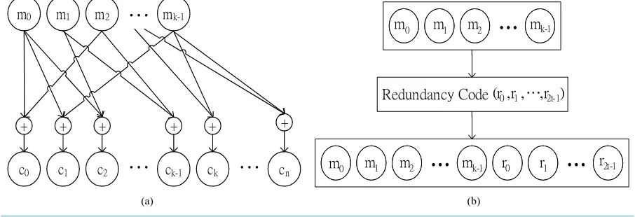
Forward Error Correction (FEC) codes have been widely used in today’s unreliable communication system, such as wireless networks, to reduce bit error rate (BER). The basic principle behind FEC is to generate redundancy code by encoding the user data; the former is then appended to the latter before transmission. At the receiver, user data together with the redundancy code are examined so that a certain pattern of bit errors can be corrected. FEC is composed of two categories, convolution code (CC) and block code (BC) [3]. The former has been ap-plied to the transmission for continuous data, such as video streaming. Encoding process in CC requires rela-tively larger memory to store the previous, the current, and the upcoming information. As shown inFigure 1(a), each symbol in the k symbols,
(
m m0, 1,,mk−1)
is Exclusive-ORed with the previous or the upcomingsym-bols. As a result, n symbols
(
c c0, 1,,cn−1)
are produced from k symbols. BC, on the other hand, has been usedin encoding discrete data on the basis of block by block. Thus, BC is more applicable to a sensor network, where data, such as temperature, moisture, etc., are collected discretely in a block size. The basic idea behind BC is to encode k-symbol information with a division operation. Redundancy codes with n-k symbols,
(
r r0, ,1,rn k− −1)
,are generated after the division operation. Before the transmission to an upper stream node, the n-k symbols are attached to the original k symbols, as shown in Figure 1(b).
2.2. RS Encoding
1) It is well known that Reed-Solomon (RS) code is one of the most popular block codes. RS Code is usually represented by GF
( )
2m, where GF is the Galois Field [19] and m denotes the number of bits in a symbol. Al-ternatively, RS code can be represented by (n, k), where n=2m−1 denotes the total number of symbols en-coded, k is number of symbols for user data, and (n-k) denotes the number of redundancy symbols. Hence,
2
n k
t= − denotes the number of erroneous symbols that can be corrected.
2) Let us briefly review the operations of RS codes. Before a message is transmitted using RS encoding, the message is segmented into a number of m-bit symbols. The k m-bit symbols can be represented by a polynomial:
( )
1 1 2 11 2 1 0
0 .
k i k k
i k k i
M X =
∑
=− m X =m−X − +m− X − + + m X +m A generator polynomial, G X( )
, is defined as( )
2 1(
) (
)(
) (
)
0 1 2 1
0 ,
t
i t
i
G X =
∏
=− X−α = X−α X−α X−α − which is used to calculate a parity polynomial,( )
P X ; i.e., P X
( )
=M X X( )
2tmodG X( )
. Finally, codeword, C X( )
, is calculated by( )
( )
2t( )
C X =M X X +P X . The coefficients of polynomial C X
( )
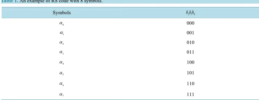
are the final encoded data to be transmit-ted.3) For example, a RS code has m=3 and k=3 or (n, k) = (7, 3); i.e., a message is segmented into a num-
[image:3.595.86.539.555.710.2](a) (b)
Figure 1. Convolution code versus block code. (a) Convolution Code; (b) Block Code.
m0 m1 m2 mk-1
c0 c1 c2 ck-1 ck cn
+ + + + + +
Redundancy Code
m0 m1 m2 m
m0 m1 m2 m
r0 r1 r
(r0
, r1, … r, 2-1t )
ber of 3-bit symbols. The 8 different symbols and their binary representations are shown inTable 1. We assume the original user data is 9 bits: 001 010 011. Since a symbol consists of 3 bits and
(
)
2(
7 3)
2 2.t= n−k = − = From Table 1, the three symbols are represented by α α α1 2 3. Thus, we have
( )
2 2 11 2 3
0
i i i
M X =
∑
= m X =α X +α X +α and( )
3(
)(
)(
)(
)
4 3 20 1 2 3 3 0 1 3
0
i
G X =
∏
= X−α X−α X−α X−α =X +α X +α X +α X+α .Parity polynomial is computed as P X
( )
=M X X( )
4mod 0G X( )
= X3+0X2+α0X+α3. Thus,( )
( )
4( )
6 5 4 3 21 2 4 0 0 1 4.
C X =M X X +P X =α X +α X +α X +α X +α X +α X+α From Table 1, we know the
encoded data to be transmitted are 001 010 100 000 000 001 100.
2.3. RS Decoding
Due to noise or interference, data may encounter bit errors over wireless link. Let R(X) be the data received, C(X) be the data transmitted, and E(X) be the data in error. Thus, we have, R X
( )
=C X( ) ( )
+ X . To determine whether or not R(X) requires any corrections, we have to compute E(X) by their syndromes:(
S S1, 2,,S2t)
. From Equation (1), if Si =0, then E( )
αi =0, which implies R( )
αi =C( )
αi ; i.e., no bit errors occur. Other-wise,bit errors occur and E(X) is computed.( )
( ) ( )
, 1, 2, ,2i i i i
S =R α =C α +E α i= t (1)
If bit errors do occur, error locations and error values are required computation. Assume there are v errors appear at the locations, Xl1,Xl2,,Xlv. That is, E X
( )
=Xl1+Xl2+ + Xlv and their syndromes can be expressed as in Equation (2).( )
( )
( )
1 2
1 1 1 1 1
1 2
2 2 2 2 2
1 2
2 2 2 2 2
l l l
l l l
l l l
t t t t t
S E
S E
S E
ν
ν
ν
α α α α
α α α α
α α α α
= = + + +
= = + + +
= = + + +
(2)
Next, if we can find
(
α αl1, l2,,αlv)
such that all syndromes are equal to zero, then the errors can be located from the exponents of α. Let βi =αli, 1, 2,∀ =i ,v. The syndromes can be expressed as in Equation (3).
1 2
1 1 1 1 1 1
1 2
2 2 2 2 1 2
1 2
2 2 2 2 1 2
i i
i i
i t t t t i t
S
S
S
ν ν
ν ν
ν ν
β β β β
β β β β
β β β β
=
=
=
= + + + =
= + + + =
= + + + =
∑
∑
∑
[image:4.595.85.538.539.715.2](3)
Table 1. An example of RS code with 8 symbols.
Symbols b b b2 1 0
0
α 000
1
α 001
2
α 010
3
α 011
4
α 100
5
α 101
6
α 110
7
Thus, the polynomial of error locations can be expressed as shown in Equation (4).
( )
(
)
11 1
11 1
i i
X ν νXν ν Xν X
σ β σ σ − σ
− =
=
∏
+ = + + + + (4)To compute σi, we let
( )
1
i
X = β − and substitute it into Equation (4). Next, we let σ
( )
X =0, which re- sults to Equation (5), where i=1, 2,,v and l=1, 2,, 2t−v. From Equation (5), we can derive Equation (6).( )
( )
1( )
1 0
l l l
i i i
v
ν ν
σ β +σ − β + ++ β + = (5)
( )
( )
( )
(
1)
1
1 0
l l l
i i i
v i
ν ν
ν
σ β σ − β + β +
= + + + =
∑
(6)Expanding Equation (6), the result is shown in Equation (7).
( )
( )
1( )
1
1 1 1 0
l l l
i i i
i i i
ν
ν ν ν
ν ν
σ β σ − β + β +
= + = + + = =
∑
∑
∑
(7)From Equation (3) and Equation (7), we can derive Equation (8).
1 1 0
l l l
S S S
ν ν ν
σ +σ − + + + + = (8)
Substituting l=1, 2,, 2t−v to Equation (8), we have derive Equation (9).
1 2 1 1 1
2 2 1 1 1 2
2t 2t 1 1 2t1 1 2t
S S S S
S S S S
S S S S
ν ν ν ν
ν ν ν ν
ν ν ν ν
σ σ σ
σ σ σ
σ σ σ
− + − + + − − + − − + + + = − + + + = − + + + = − (9)
Equation (9) can be expressed by a matrix equation as shown in Equation (10). By applying the operation of inverse matrix, we can compute σi.
1 2 1
2 3 1 1 2
1 2t1 1 2
S S S S
S S S S
S S S S
ν ν ν
ν ν ν
ν ν ν
σ σ σ + + − + + − − − = − (10)
Substituting σi to Equation (4), we can find
i
β ;i.e., the error locations. To compute error values, we de-fine them as e ev′ ′, v−1,,e1′ as shown in Equation (11).
( )
( )
( )
( )
11 1
R X =C X +E X′ =C X +e Xν′ ν +eν′− Xν− + + e X′ (11)
Let X =α α1, 2,,αv. By substituting X to Equation (11), we have derive Equation (12).
1
1 1 1 1 1 1
1
2 1 2 1 2 2
1
1 1
e e e S
e e e S
e e e S
ν ν
ν ν
ν ν
ν ν
ν ν
ν ν ν ν ν ν
α α α
α α α
α α α
− − − − − − ′ + ′ + + ′ = ′ + ′ + + ′ = ′ + ′ + + ′ = (12)
Since Equation (12) has v equations and v unknown, it is easy to compute v. Finally, errors can be cor-rected by adding error values v to their corresponding positions. At last, let us give an example. We assume the received data = 001 010 000 011 000 001 011, which can be represented by a polynomial
( )
6 5 4 3 21 2 0 3 0 1 3.
R X =α X +α X +α X +α X +α X +α X+α We then calculate the 4 syndromes,
( )
1 1 2
S =R α =α , S2=R
( )
α2 =α1, S3=R( )
α3 =α6, and S4=R( )
α4 =α6. By substituting them intoEqua-tion (10), we obtain the error locaEqua-tions as shown in EquaEqua-tion (13).
3 5 2 6
5 6 1 0
α α σ α
α α σ
=
1 0 0
2 6
0 5 6
1 0
α α α
σ α
α α α
σ
= =
(14)
By multiplying an inverse matrix on both sides in Equation (13), we have derive Equation (14). Next, if we substitute σ2 and σ1 to an error-location polynomial, we have
( )
2
0 6 0
X X X
σ =α +α +α . Now, we can de-rive σ α
( )
0 =α6, σ α( )
1 =α2 , σ α( )
2 =α6, σ α =( )
3 0 , σ α =( )
4 0, σ α( )
5 =α2 , and σ α( )
6 =α0 . Hence, the two error locations are found, which show us the third and the fourth symbols are in error. To com-pute these two error values, we need to comcom-pute S1 and S2 first, as shown in Equation (15). Thus, the twoerror values can be computed from Equation (16).
3 4
1 1
1 1
3 4
2 2
2 2
e S
e S
α α α α
′
= ′
(15)
2 5 3
1 2
0 4 3
2 1
e
e
α α α α
α α α α
′
= =
′
(16)
Since E X
( )
=α3X4+α3X3, the received data are corrected as,( )
( )
( )
6 5 4 3 21 2 3 0 0 1 3,
C X′ =R X +E X =α X +α X +α X +α X +α X +α X+α which in binary representation is 001 010 011 000 000 001 011.
3. Packet Interleaving Scheme
3.1. WSN with Multi-Hop Tree Structure
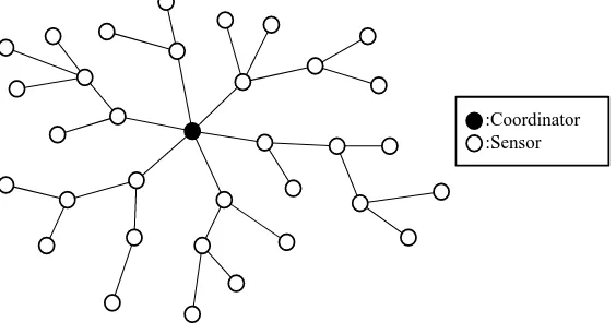
In a wireless sensor network (WSN), a coordinator is the sink which gathers all the data collected from other distant sensor nodes. To facilitate data gathering from all the sensor nodes, it is very constructive that the coor-dinator and the sensor nodes will collaborate to build a multi-hop tree structure (MTS), as shown inFigure 2. In an MTS-based WSN, data collected by a sensor node will be forwarded hop-by-hop to the coordinator. Thus, by fully utilizing a branch node of the MTS, in this paper, we propose a packet interleaving scheme (PIS) based on RS codes to reduce the impact of burst errors on packet uncorrectable probability.
3.2. Packet Interleaving
[image:6.595.174.456.552.705.2]In the proposed PIS, packets collected by a sensor node are classified into two different types: high-reliability required (HRR) packet and non-HRR packet. An HRR packet is defined as a packet which requires for retrans-mission, if uncorrectable burst errors exist. Payload in an HRR packet consists of numerical data, such as tem-perature, moisture, luminance, etc. This type of packet has relatively shorter data length (usually, a couple of bytes) and each uncorrectable HRR packet requires for retransmission. Hence, it is better to employ a short-er-length symbol (in this paper, we use m = 4) to encode an HRR packet with shorter data length. On the other
Figure 2. WSN with multi-hop tree structure. :Coordinator
hand, payload in a non-HRR packet consists of non-numerical data, such as video, audio, etc. This type of pack-et has relatively longer data length (usually, in the order of kilo bytes) and each uncorrectable non-HRR packpack-et may not require for retransmission. Thus, it is better to employ longer-length symbol (in this paper, we use m = 8) to encode a non-HRR packet with longer data length.
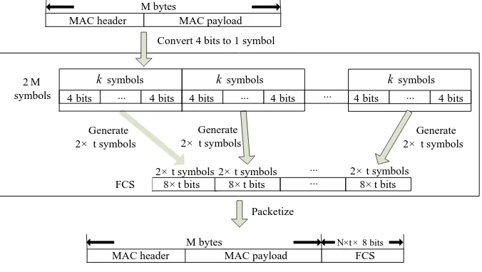
As it is illustrated in Figure 3, an HRR packet is encoded with a shorter-length RS symbol (i.e., m = 4). First,
an M-byte MAC-layer header and payload is converted to
(
8)
2 4M
M
×
= symbols on the basis of 4 bits per
symbol. Thus, we have the length of a codeword is n, where n=2m− =1 24− =1 15, the number of symbols for user data in a codeword is k, where k= − × =n 2 t 15 2− ×t, and the number of symbols for redundancy code in a codeword is 2×t. Let N 2M
k
= , which denotes the number of codeword required for encoding the M-byte packet (header plus payload). The total redundancy code (or FCS) is therefore equal to N× ×2 t symbols, or
(
)
2 4 8
N× × ×t = × ×N t bits.
Similarly, as it is illustrated in Figure 4, a non-HRR packet is encoded with a longer-length symbol (m = 8).
An M-byte MAC-layer header and payload is converted to
(
8)
8
M
M ×
= symbols on the basis of 8 bits per
symbol. Since the length of a codeword, n=2m− =1 28− =1 255
bytes, which is much greater than the maxi-mum length of a packet, which is 127 bytes in a WSN, a codeword is sufficiently enough to encode a MAC-layer packet in a WSN. Thus, the length of redundancy code (or FCS) is equal to 2×t bytes.
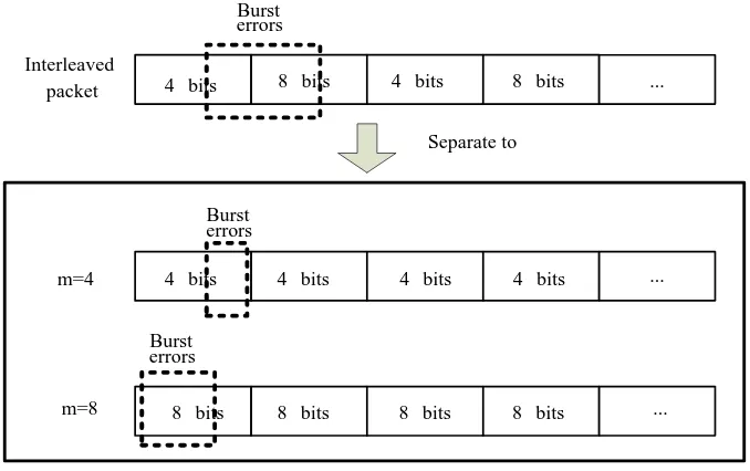
When both an HRR and a non-HRR packet are received by a branch node in a tree-structured WSN, these two packets are interleaved on a symbol-by-symbol basis, as shown inFigure 5. The interleaved packet is then for-warded to an upper stream node, which performs decoding and correction process. However, as shown in Fig-ure 6, an interleaved packet may not be correctable, if it encounters burst errors where the number of total errors is greater than t. In the proposed PIS, by separating the interleaved single packet back to their original two pack-ets, each individual packet may become correctable. This is because the number of errors in each separated packet is highly possible to be smaller than t.
4. Mathematical Model and Analysis
[image:7.595.145.483.514.705.2]In RS codes, whether or not a coded packet is correctable is mainly determined by the number of erroneous sym-bols. In this section, to study the robustness and the error-correction capability of the proposed PIS, we build two mathematical models for comprehensive numerical simulations. The first one is referred to as uniform bit error model (UBEM), while the second one is referred to as on-off bit error model (OBEM). The first model assumes the errors occur evenly on the coded packets. The second model assumes the errors may occur continuously
Figure 3. An HRR packet encoded with a shorter-length symbol (m = 4).
MAC payload MAC header
M bytes
FCS
...
FCS Generate 2× t symbols
Packetize MAC payload
MAC header
... ...
...
Generate
2×Generate t symbols
...
M bytes
Convert 4 bits to 1 symbol
symbols
k ksymbols
2 M
symbols 4 bits 4 bits 4 bits 4 bits
symbols k
4 bits 4 bits
2× t symbols 2× t symbols ... 2× t symbols 2× t symbols
8× t bits 8× t bits 8× t bits
Figure 4. A non-HRR packet encoded with a longer-length symbol (m = 8).
Figure 5. Packet interleaving on a symbol-by-symbol basis.
Figure 6. Burst errors dispersed on two symbols.
in a burst length.
4.1. UBEM
Let PUB be_ and PUB_se denote the probability of bit errors and the probability of symbol errors, respectively.
Since any bit errors occur in a symbol may result in a symbol error and each symbol has m bits, we can derive
M bytes
M symbols M bytes
MAC payload MAC header
Generate 2× t symbols
Packetize
...
Convert 1 byte to 1 symbol
8 bits 8 bits 8 bits 8 bits 8 bits
2 × t symbols
FCS
2 × t bytes
MAC header MAC payload FCS
...
...
Symbol
interleaving ...
m=4
m=8
4 bits 4 bits 4 bits
4 bits 4 bits 8 bits 8 bits 8 bits
8 bits 8 bits
m=4
m=8
... Separate to
...
... 4 bits
4 bits 4 bits 4 bits 4 bits
Interleaved packet
Burst errors
Burst errors
8 bits
8 bits 8 bits 8 bits 8 bits
Burst errors
_
UB se
P directly from PUB be_ , as shown in Equation (17).
(
)
_ 1 1 _
m UB se UB be
P = − −P (17)
Next, let us define two more parameters, NS and NC. The first parameter denotes the number of symbols
in a codeword and the second parameter denotes the number of codeword in a packet. Hence, the uncorrectable probability of a codeword
(
PUB cuc_)
, can be derived as shown in Equation (18).(
) (
)
_ 1 0 _ 1 _
S
i N i
t s
UB cuc i UB se UB se
N
P P P
i
− =
= − × × −
∑
(18)In Equation (18), we know in a codeword if the number of symbol errors is smaller than t, then the codeword is correctable. Thus, the uncorrectable probability of a codeword can be summed up from i=0 to t, since there
are Ns
i
different types of errors. Next, let us define PUB_puc as the packet uncorrectable probability.
Since there are NC codeword in a packet, we can derive PUB_puc as shown in Equation (19).
(
)
_ 1 1 _
C
N UB puc UB cuc
P = − −P (19)
4.2. OBEM
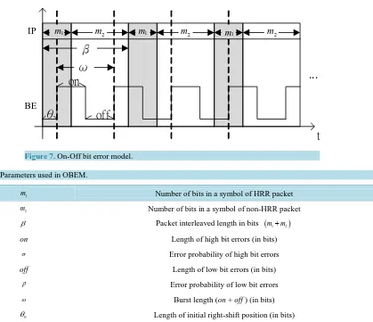
The on-off bit error model (OBEM) is illustrated inFigure 7. All the parameters used in the analysis are defined inTable 2. A burst error (BE) period is defined as two consecutive bit error intervals where high bit errors ap-
[image:9.595.119.538.353.714.2]Figure 7. On-Off bit error model.
Table 2. Parameters used in OBEM.
1
m Number of bits in a symbol of HRR packet
2
m Number of bits in a symbol of non-HRR packet
β Packet interleaved length in bits (m1+m2)
on Length of high bit errors (in bits)
σ Error probability of high bit errors
off Length of low bit errors (in bits)
ρ Error probability of low bit errors
ω Burst length (on + off ) (in bits)
0
θ Length of initial right-shift position (in bits)
t
ω
β
on
off
θ
...
1
m m2 m1 m2 m1 m2
IP
pear first and then followed by low bit errors. Notice that θ0 is defined as the length of right-shift position for
an initial BE period; θ0 =0 implies that no gap exists between the beginning of an interleaved packet and the
beginning of the first BE period.
First, we define POB_se as the symbol-error probability in OBEM. An interleaved packet (IP) and a burst er-ror (BE) may have different lengths; here we assume the former has a length of β bits
(
β =m1+m2)
andthe later has a length of
ω
bits(
ω=on+off)
. Since every symbol in an IP may encounter different positions of bit errors, we have to analyze the bit error positions of a symbol before we can compute the symbol-error probability. To compute the error probability of the αthsymbol, we define (i) m1s = the distance between the
first bit of m1 and the first bit of an IP, and (ii) m1e = the distance between the last bit of m1 and the first bit
of an IP. Similarly, we define m2s and m2e for m2. Thus, m1s, m1e, m2s, and m2e can be computed as
shown in Equation (20), (21), (22), and (23), respectively.
1s
m = ×α β (20)
1e 1 1
m = × +α β m − (21)
2s 1
m = × +α β m (22)
(
)
2e 1 1
m = α+ × −β (23)
For simplicity, the four parameters, m1s, m1e, m2s, and m2e are generalized to mij, where i=1, 2 and
,
j=s e. Let θ denote the length of right-shift position between an IP and a BE at the αth
symbol. Let Ωmij
denote the length of right-shift position for m1s, m1e, m2s, and m2e at the th
α symbol. Thus, we can compute θ and Ωmij as shown in Equation (24) and (25), respectively.
0
header length
header length mod
θ θ ω ω
ω
= + × −
(24)
1 1 ij
ij m
m
ω θ ω
+ Ω = − × +
(25)
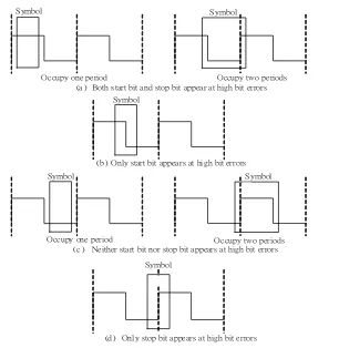
After we found the right-shift position between an IP and a BE, we can categorize the symbol errors into four cases, as illustrated from Figure 8(a) toFigure 8(d). Case 1 in Figure 8(a) shows whether or not a symbol may occupy one BE or two BE periods, their start bit and stop bit of a symbol all appear at the high-bit-error interval. Case 2 inFigure 8(b) shows only the start bit of a symbol appears at the high-bit-error interval. Case 3 in Fig-ure 8(c) shows whether or not a symbol may occupy one BE or two BE periods, neither the start bit nor the stop bit appear at the high-bit-error interval. Finally, Case 4 in Figure 8(d) shows only the stop bit of a symbol ap-pears at the high-bit-error interval. Actually, the four different cases of symbol errors can be constrained by eight inequalities with four parameters, mij, Ωmij, on, and
ω
. These eight inequalities (two inequalities foreach case) are shown inTable 3. Once we identify the four cases of symbol errors, we can compute the symbol- error probability. Since one codeword consists of Ns symbols, we define POB_se
( )
α α, =0,1,,Ns −1, as the symbol-error probability of the αthsymbol. Let
σ
denote the error probability of high bit errors and ρ denote the error probability of low bit errors. Let Nσ represent the number of bits with errors in a symbol andNρ represent the number of bits without errors in a symbol. We can compute POB_se
( )
α as shown in Equa-tion (26).( )
(
)
(
)
_ 1 1 1
N N OB se
P α = − −σ σ× −ρ ρ (26)
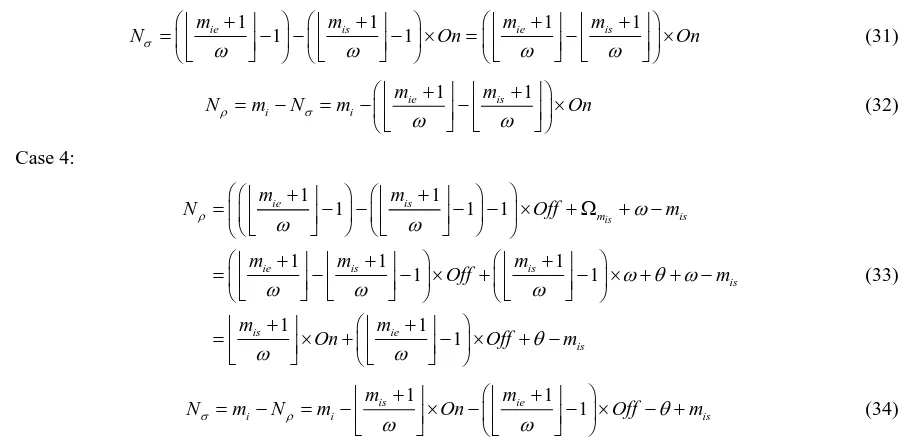
Now, we can compute Nσ and Nρ for case 1 as shown in Equation (27) and (28), case 2 as shown in Eq-uation (29) and (30), case 3 as shown in EqEq-uation (31) and (32), and case 4 as shown in EqEq-uation (33) and (34), respectively.
Case 1:
1 1 1 1
1 1
ie is ie is
m m m m
Nρ Off Off
ω ω ω ω
+ + + +
= − − − × = − ×
Figure 8. Four cases of symbol errors in terms of the start and stop bits.
Table 3. Four cases of symbol errors with 8 constraints.
Case Conditions
1 Ω ≤mis mis< Ω +mis On and Ω ≤mie mie< Ω +mie On
2 Ω ≤mis mis< Ω +mis On and Ω +mie On ≤mie< Ω +mie ω
3 Ω +mis On ≤mis< Ω +mis ω and Ω +mie On ≤mie< Ω +mie ω
4 Ω +mis On ≤mis< Ω +mis ω and Ω ≤mie mie< Ω +mie On
1 1
ie is
i i
m m
Nσ m Nρ m Off
ω ω
+ + = − = − − ×
(28)
Case 2:
1 1
1 1
1 1 1
1
1 1
1
is
ie is
m is
ie is is
is
ie is
is
m m
N On On m
m m m
On On m
m m
On Off m
σ ω ω
ω θ
ω ω ω
θ
ω ω
+ +
= − − − × + Ω + −
+ + +
= − × + − × + + −
+ +
= × + − × + −
(29)
1 1
1
ie is
i i is
m m
Nρ m Nσ m On Off θ m
ω ω
+ +
= − = − × − − × − +
(30)
Occupy one period
Only start bit appears at high bit errors
Symbol
Symbol
Symbol
Occupy two periods Symbol
Symbol
Neither start bit nor stop bit appears at high bit errors Symbol
Both start bit and stop bit appear at high bit errors (a )
(b )
(c )
[image:11.595.90.541.422.746.2]Case 3:
1 1 1 1
1 1
ie is ie is
m m m m
Nσ On On
ω ω ω ω
+ + + + = − − − × = − ×
(31)
1 1
ie is
i i
m m
Nρ m Nσ m On
ω ω
+ + = − = − − ×
(32)
Case 4:
1 1
1 1 1
1 1 1
1 1 1 1 1 is ie is m is
ie is is
is
is ie
is
m m
N Off m
m m m
Off m
m m
On Off m
ρ ω ω ω
ω θ ω
ω ω ω
θ
ω ω
+ +
= − − − − × + Ω + −
+ + + = − − × + − × + + − + + = × + − × + − (33) 1 1 1 is ie
i i is
m m
Nσ m Nρ m On Off θ m
ω ω
+ +
= − = − × − − × − +
(34)
By substituting Nσ and Nρ back to Equation (26), we can now summarize POB se_
( )
α for the fourdif-ferent cases of symbol errors as shown inTable 4.
After we compute the symbol-error probability for the four different cases, our next step is to derive the un-correctable probability of a codeword and the unun-correctable probability of a packet. We know there are NC
codeword in a packet and the uncorrectable probabilities of the NC codeword are all different. Let
( )
_ , 0,1, , 1
OB cuc c
P l l= N − , denote the uncorrectable probability of the lth codeword and let POB_puc denote
the uncorrectable probability of a packet. By using the combination theory of probabilities, we can derive
( )
_ OB cuc
P l and POB_puc as shown in Equation (35) and (36), respectively.
( )
1 1(
) (
)
_ _ _
0 0 0
1 1
ij ij
i
k
k k
t r N r
k k k
OB cuc ij OB se OB se i j k k
N
P l P P
r
τ− λ− −
= = = = − × × −
∑ ∑ ∏
(35)( )
(
)
1
_ 1 0 1 _
C
N
OB puc l OB cuc
P = −
∏
= − −P l (36)5. Numerical Simulations
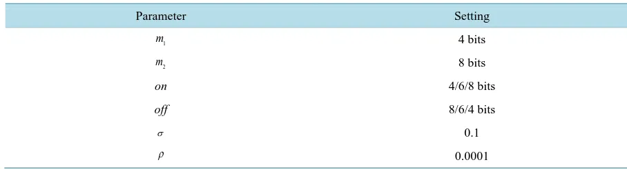
[image:12.595.89.540.98.318.2]In OBEM, to study the influences of the four parameters, (i) the length of high bit errors (i.e., the On period), (ii) the length of low bit errors (i.e., the Off period), (iii) the right-shift position (i.e., θ), and (iv) the number of correctable symbols (i.e., t), on the packet uncorrectable probability (i.e., 𝑃𝑃𝑂𝑂𝑂𝑂_𝑝𝑝𝑝𝑝𝑝𝑝), we perform comprehensive numerical simulation. Table V shows the parameters and their setting used in the simulation. FromTable 5, we can observe that an On-Off period is fixed to 12 bits. Within the 12 bits, the On period is varied among three different lengths; shorter length (4 bits), equal length (6 bits), and longer length (8 bits). The length of Off period is varied from the other directions (i.e., from longer to shorter length).
Table 4. Four cases of symbol-error probabilities.
Case POB se_ ( )α
1 1 (1 )i ie1 is1 (1 ) ie1 is1
m m m m
m Off Off
ω ω ω ω
σ − + − + × ρ + − + ×
− − × −
2 ( ) 1 1 1 ( ) 1 11
1 1 1
ie is ie is
is i is
m m m m
On Offθm m On Offθm
ω ω ω ω
σ +× + +− × + − ρ − +× − +− × − +
− − × −
3 1 (1 ) ie1 is1 (1 )i ie1 is1
m m m m
On m On
ω ω ω ω
σ + − + × ρ − + − + ×
− − × −
4 ( ) 1 11 ( ) 1 11
1 1 i is ie is 1 is ie is
m m m m
m ω On ω Offθm ω On ω Offθm
σ − +× − +− × − + ρ +× − +− × + −
Table 5. Parameter settings.
Parameter Setting
1
m 4 bits
2
m 8 bits
on 4/6/8 bits
off 8/6/4 bits
σ 0.1
ρ 0.0001
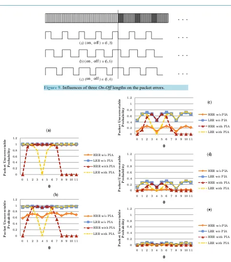
Prior to studying the influences of the three different On-Off lengths on packet uncorrectable probability, we illustrate three scenarios inFigure 9. When the length of On period is shorter, as shown inFigure 9(a), an HRR packet encoded with a shorter length of symbol (m = 4, dark-shaded portion) completely falls in the Off period, while a non-HRR packet encoded with a longer length of symbol (m = 8, light-shaded portion) just has a few bits fall in the Off period. When the length of the On period is increased to 6 bits, which is equal to the length of the Off period, as shown in Figure 9(b), half of the HRR packet falls in the On period. The error-bit coverage for an HRR packet becomes even worse when the On period is increased to 8 bits, as shown inFigure 9(c). As it can be seen, a whole symbol of an HRR packet is now covered by the On period, while only half of a symbol of a non-HRR packet is covered by the On period.
Impact of Correctable Symbols
First, we are interested in studying the impact of increasing the number of correctable symbols when the length of high bit errors is shorter than the length of low bit errors; i.e., On = 4 bits and Off = 8 bits. As shown in Fig-ures 10(a) to 10(e), we observe the variations of packet uncorrectable probability
(
POB_puc)
when the right-shiftposition
( )
θ is increased from 0 to 11 bits and the number of correctable symbols (t) is increased from 1 to 5. From Figure 10, we can observe that both the packet uncorrectable probabilities(
POB_puc)
of HRR andnon-HRR curves drop off very quickly, when the number of correctable symbols (t) is increased from 1 to 5. Additionally, we can observe that he curves of POB_puc with PIS (the two dashed lines) are much lower than the curves of POB_puc without using PIS (the two solid lines). The improvement of POB_puc by using PIS is more significant when t is small, which is quite beneficial for reducing packet overhead, since the number of redun-dancy bits in RS codes can be shorter. Another noticeable phenomenon is that although when θ is smaller than 7, the curves of HRR with PIS are completely inverted to the curves of non-HRR with PIS, the curves of HRR with PIS do drop to zero when θ is larger than 7. In other words, on average we have come out a result; i.e., the packet uncorrectable probability of HRR with PIS is significantly lower than that of non-HRR with PIS.
FromFigure 11(a) toFigure 11(e), we show the packet uncorrectable probabilities when the on period (6 bits) is equal to the Off period (6 bits). It is not surprising to notice that, for the corresponding t values (t = 1 to 5), the four curves inFigure 11 are much higher than those four curves in Figure 10. The reason is quite straightfor-ward, since the period of high bit errors (i.e., the On period) is increased from 4 bits to 6 bits. However, on av-erage the proposed PIS can effectively reduce packet uncorrectable probability, as it is compared to the curves without using PIS. In particular, we can observe that, no matter what the value t is, the curves of HRR with PIS can be reduced to near zero when θ is larger than 7. Additionally, we observe that a side effect could occur. That is, the curves of non-HRR with PIS cannot be reduced very significantly, as they are compared to those curves in Figure 10. This is because no matter how we adjust the right-shift position
( )
θ , a non-HRR packet will be affected by the on period since the latter has been increased from 4 bits to 6 bits.Figure 9. Influences of three On-Off lengths on the packet errors.
Figure 10. Variations of packet uncorrectable probability (on is smaller than off).
is no advantage achieved by using the proposed PIS.
FromFigure 13(a) toFigure 13(c), we show the comparisons in packet uncorrectable probabilities between UBEM and OBEM. First, we observe that in UBEM it does not make any big difference whether or not using the proposed PIS, since in UBEM every bit receives the same error probability. Second, we observe that packet uncorrectable probability in UBEM is relatively higher than that in OBEM. Notice that the curves of UBEM and the curves of OBEM vary along with the following two parameters: (i) when the number of correctable symbols (t) increases from 1 to 5, the curves of UBEM dissever very quickly from those of OBEM; and (ii) when the right-shift position
( )
θ increases from zero to 8 bits, the gap between these two models becomes smaller. Since OBEM is more reactive to a real word than UBEM, it is rewarding to know that the proposed PIS can reduce packet uncorrectable probability in OBEM more significantly than that in UBEM. Another noticeable re-, (c) (on, off ) = (84) (b) (on, off ) = (6, 6) (a) (on, off ) = (4, 8)
‧‧‧ ‧‧‧ ‧‧‧ ‧‧‧ 1 0 0.2 0.4 0.6 0.8 1 1.2
0 1 2 3 4 5 6 7 8 9 10 11
P ac ket U n co rr ec ta bl e P robabil it y θ
HRR w/o PIA LRR w/o PIA HRR with PIA LRR with PIA
0 0.2 0.4 0.6 0.8 1 1.2
0 1 2 3 4 5 6 7 8 9 10 11
P ac ket U n co rr ec ta bl e P robabil it y θ
HRR w/o PIA LRR w/o PIA HRR with PIA LRR with PIA
0 0.2 0.4 0.6 0.8 1 1.2
0 1 2 3 4 5 6 7 8 9 10 11
P ac ket U n co rr ec ta bl e P robabil it y θ
HRR w/o PIA LRR w/o PIA HRR with PIA LRR with PIA
0 0.2 0.4 0.6 0.8 1 1.2
0 1 2 3 4 5 6 7 8 9 10 11
P ac ket U n co rr ec ta bl e P robabil it y θ
HRR w/o PIA LRR w/o PIA HRR with PIA LRR with PIA
0 0.2 0.4 0.6 0.8 1 1.2
0 1 2 3 4 5 6 7 8 9 10 11
P ac ket U n co rr ec ta bl e P robabil it y θ
HRR w/o PIA LRR w/o PIA HRR with PIA LRR with PIA
(a)
(b)
(c)
(d)
Figure 11. Variations of packet uncorrectable probability (on is equal to off).
Figure 12. Variations of packet uncorrectable probability (on is larger than off).
2 0 0.2 0.4 0.6 0.8 1 1.2
0 1 2 3 4 5 6 7 8 9 10 11
P ac ket U n co rr ec ta bl e P robabil it y θ
HRR w/o PIA LRR w/o PIA HRR with PIA LRR with PIA
0 0.2 0.4 0.6 0.8 1 1.2
0 1 2 3 4 5 6 7 8 9 10 11
P ac ket U n co rr ec ta bl e P robabil it y θ
HRR w/o PIA LRR w/o PIA HRR with PIA LRR with PIA
0 0.2 0.4 0.6 0.8 1 1.2
0 1 2 3 4 5 6 7 8 9 10 11
P ac ket U n co rr ec ta bl e P robabil it y θ
HRR w/o PIA LRR w/o PIA HRR with PIA LRR with PIA
0 0.2 0.4 0.6 0.8 1 1.2
0 1 2 3 4 5 6 7 8 9 10 11
P ac ket U n co rr ec ta bl e P robabil it y θ
HRR w/o PIA LRR w/o PIA HRR with PIA LRR with PIA
0 0.2 0.4 0.6 0.8 1 1.2
0 1 2 3 4 5 6 7 8 9 10 11
P ac ket U n co rr ec ta bl e P robabil it y θ
HRR w/o PIA LRR w/o PIA HRR with PIA LRR with PIA
(a)
(b)
(c)
(d)
[image:15.595.103.528.155.698.2]Figure 13. Packet uncorrectable probability in UBEM vs in OBEM. (a) (On, Off, θ) = (4, 8, 0); (b) (On, Off, θ) = (6, 6, 8); (c)
(On, Off, θ) = (4, 8, 8)
sult is that no matter how we increase the period of high bit errors (i.e., we increase the on period from 4 bits in 13(a) to 6 bits in 13(b), and finally to 8 bits in 13(c)), HRR with PIS in OBEM always exhibits the lowest packet uncorrectable probability (near zero, in some cases). The relatively lower packet uncorrectable probability for HRR packets has demonstrated that the proposed PIS can successfully protect HRR packets from burst errors, while at the same time it does not sacrifice non-HRR packets from large uncorrectable bit errors.
6. Conclusion
In this paper, we have presented a packet interleaving scheme (PIS) using RS code to reduce packet uncorrecta-ble probability under burst errors in wireless sensor networks. In PIS, the collected data are classified into HRR and non-HRR. An HRR packet is encoded with a shorter RS symbol, while a non-HRR packet with a longer RS symbol. One of the contributions of this paper is right in that an HRR and a non-HRR packet are interleaved on a symbol-by-symbol basis, which effectively disperses the burst errors among an interleaved packet. Conse-quently, the packet uncorrectable probability of an HRR packet can be significantly reduced. In the performance evaluation, we built two mathematical models, UBEM and OBEM. From the thorough numerical simulations, we have demonstrated that, no matter how we adjust the period of high bit errors, the proposed PIS behaves more resilient to burst errors in OBEM than in UBEM. Finally, we have revealed that, by carefully adjusting the period of high bit errors and the right-shift positions, the proposed PIS can reduce the uncorrectable probability of HRR packets to near zero.
Acknowledgements
The authors would like to thank the reviewers, whose valuable comments helped improve the presentation of this paper. Additionally, the authors would like to thank Prof. Tsang-Ling Sheu’s assistant, Miss Yi-Ying Ke for her cautious redrawing of the figures which helped improve the quality of the paper. This study is supported under the three grant numbers: (1) NSC 102-2221-E-110-036-MY2 of MoST, Taiwan, (2) 103-EC-17-A-03-S1- 214, of MOEA, Taiwan, and (3) NHRI-EX103-10142EI, Taiwan.
References
[1] Barac, F., Yu, K., Gidlund, M., Akerberg, J. and Bjrkman, M. (2012) Towards Reliable and Lightweight
Communica-4
0 0.2 0.4 0.6 0.8 1 1.2
1 2 3 4 5
P
ac
ket
U
n
co
rr
ec
ta
bl
e
P
robabil
it
y
t
HRR (UBEM) LRR (UBEM) HRR w/o PIA LRR w/o PIA HRR with PIA LRR with PIA
0 0.2 0.4 0.6 0.8 1 1.2
1 2 3 4 5
P
ac
ket
U
n
co
rr
ec
ta
bl
e
P
robabil
it
y
t
HRR (UBEM) LRR (UBEM) HRR w/o PIA LRR w/o PIA HRR with PIA LRR with PIA
0 0.2 0.4 0.6 0.8 1 1.2
1 2 3 4 5
P
ac
ket
U
n
co
rr
ec
ta
bl
e
P
robabil
it
y
t
HRR (UBEM) LRR (UBEM) HRR w/o PIA LRR w/o PIA HRR with PIA LRR with PIA
(a)
(b)
tion in Industrial Wireless Sensor Networks. Proceedings of theINDIN 2012: IEEE 10th International Conference on Industrial Informatics, Beijing, 25-27 July 2012, 1218-1224. http://dx.doi.org/10.1109/indin.2012.6300846
[2] Marinkovic, S. and Popovici, E. (2009) Network Coding for Efficient Error Recovery in Wireless Sensor Networks for
Medical Applications. Proceedings of the 1st International Emerging Network Intelligence, Sliema, 11-16 October
2009, 15-20. http://dx.doi.org/10.1109/emerging.2009.22
[3] Sklar, B. (2001) Digital Communications: Fundamentals and Applications. 2nd Edition, Prentice Hall, Upper Saddle
River.
[4] Chebbo, H., Abedi, S., Lamahewa, T.A., Smith, D.B., Miniutti, D. and Hanlen, L. (2010) Reliable Body Area
Net-works Using Relays: Restricted Tree Topology. Proceedings of the 2012 International Conference on Computing,
Networking and Communications (ICNC), Maui, 30 January-2 February 2010, 82-88.
http://dx.doi.org/10.1109/iccnc.2012.6167540
[5] Sampangi, R.V., Urs, S.R. and Sampalli, S. (2011) A Novel Reliability Scheme Employing Multiple Sink Nodes for
Wireless Body Area Networks. Proceedings of the 2011 IEEE Symposium on Wireless Technology and Applications
(ISWTA), Langkawi, 25-28 September 2011, 162-167. http://dx.doi.org/10.1109/iswta.2011.6089401
[6] Kim, S., Fonseca, R. and Culler, D. (2004) Reliable Transfer on Wireless Sensor Network. Proceedings of the 1st
An-nual IEEE Communications Society Conference on Sensor and Ad Hoc Communications and Networks, Santa Clara, 4-7 October 2004, 449-459.
[7] Byrne, E., Manada, A., Marinkovic, S. and Popovici, E. (2011) A Graph Theoretical Approach for Network Coding in
Wireless Body Area Networks. Proceedings of the 2011 IEEE International Symposium on Information Theory
Pro-ceedings (ISIT), Saint Petersburg, 31 July-5 August 2011. http://dx.doi.org/10.1109/isit.2011.6034156
[8] Hamada, Y., Takizawa, K. and Ikegami, T. (2012) Highly Reliable Wireless Body Area Network Using Error
Correct-ing Codes. Proceedings of the 2012 IEEE Radio and Wireless Symposium, Santa Clara, 15-18 January 2012, 231-234.
http://dx.doi.org/10.1109/rws.2012.6175351
[9] Luby, M. (2002) LT Codes. Proceedings of the 43rd Annual IEEE Symposium on Foundations of Computer Science,
Vancouver, 16-19 Novenber 2002, 271-280. http://dx.doi.org/10.1109/sfcs.2002.1181950
[10] Ishibashi, K., Ochiai, H. and Kohno, R. (2008) Embedded Forward Error Control Technique (EFECT) for Low-Rate
but Low Latency Communications. IEEE Transactions on Wireless Communications, 7, 1456-1460.
http://dx.doi.org/10.1109/TWC.2008.060573
[11] Busse, M., Haenselmann, T. and Effelsberg, W. (2007) Energy-Efficient Data Dissemination for Wireless Sensor
Net-works. Proceedings of the 5th Annual IEEE International Conference on Pervasive Computing and Communications
Workshops, White Plains, 19-23 March 2007. http://dx.doi.org/10.1109/percomw.2007.44
[12] Yu, K., Barac, F., Gidlund, M., Akerberg, J. and Bjorkman, M. (2012) A Flexible Error Correction Scheme for IEEE
802.15.4-Based Industrial Wireless Sensor Networks. Proceedings of the 2012 IEEE International Symposium on
In-dustrial Electronics (ISIE), Hangzhou, 28-31 May 2012, 1172-1177. http://dx.doi.org/10.1109/isie.2012.6237255
[13] Srouji, M.S., Wang, Z. and Henkel, J. (2011) RDTS: A Reliable Erasure-Coding Based Data Transfer Scheme for
Wireless Sensor Networks. Proceedings of the 2011 IEEE 17th International Conference on Parallel and Distributed
Systems, Tainan, 7-9 December 2011, 481-488. http://dx.doi.org/10.1109/icpads.2011.104
[14] Arrobo, G.E. and Gitlin, R.D. (2011) Improving the Reliability of Wireless Body Area Networks. Proceedings of the
33rd Annual International Conference of the IEEE Engineering in Medicine and Biology Society (EMBC), Boston, 30
August-3 September 2011, 2192-2195. http://dx.doi.org/10.1109/iembs.2011.6090413
[15] Taparugssanagorn, A., Ono, F. and Kohno, R. (2010) Network Coding for Non-Invasive Wireless Body Area Networks.
Proceedings of the 2010 IEEE 21st International Symposium on Personal, Indoor and Mobile Radio Communications Workshops, Istanbul, 26-30 September 2010, 134-138. http://dx.doi.org/10.1109/pimrcw.2010.5670413
[16] Salhi, I., Ghamri-Doudane, Y., Lohier, S. and Roussel, G. (2011) Reliable Network Coding for ZigBee Wireless
Sen-sor Networks. Proceedings of the 8th IEEE International Conference on Mobile Ad-Hoc and Sensor Systems, Valencia,
17-22 October 2011, 135-137.
[17] Kiss, Z.I., Polgar, Z.A., Stef, M.P. and Bota, V. (2012) Network Coding Solution for Improving Transmission
Relia-bility in Wireless Sensor Networks Employed in Industrial Monitoring. Proceedings of the 35th International
Confe-rence on Telecommunications and Signal Processing (TSP), Prague, 3-4 July 2012, 190-195.
http://dx.doi.org/10.1109/tsp.2012.6256280
[18] Reed, I.S. and Solomon, G. (1960) Polynomial Codes over Certain Finite Fields. Journal of the Society of Industrial
and Applied Mathematics, 8, 300-304. http://dx.doi.org/10.1137/0108018