Uncertain 2D Continuous Systems with State Delay:
Filter Design using an
H
Polynomial Approach
C.El-Kasri, A. Hmamed, E.H. Tissir
LESSI, Department of Physics, Faculty of Sciences Dhar El Mehraz, P.O. Box 1796, Fes-Atlas 30000,
Morocco
F. Tadeo
Department of Systems Engineering and Automatic Control, University of Valladolid, 47005 Valladolid,
Spain
ABSTRACT
This paper proposes a methodology to design filters that extract information from noisy signals. From a mathematical point of view, a method is used based on homogeneous polynomially parameter-dependent (HPPD) matrices of arbitrary degree. The optimal H filter is then obtained by solving a convex optimization problem using off-the-self software. To show the effectiveness of the proposed filter design methodology some examples are solved, and the solution is illustrated using computer simulations.
Keywords
Systems theory, uncertainty, delays, filtering, linear matrix inequalities (LMI).
1.
INTRODUCTION
Designing filters and observers is a well-studied problem in one-dimensional systems (see, for example, [1], [2], and references therein), and some two-dimensional systems in image processing applications (see [3] and references therein. More precisely, a solution to the H filtering problem is given in this paper for the class of two dimensional (2-D) continuous systems that are described by a Roesser state space model with both state delays and parameter uncertainties. Delays are considered L2 as they appear frequently in practical problems (see [5] and references therein). Similarly, uncertainties are inherent to any practical implementation (see [6] and references therein).
The H estimation problem has attracted much interest in the past decades within the systems theory community [24], [38]. One of the reasons is the fact that it does not require a precise knowledge of the statistics of the noisy signals, as required by alternatives approaches. This estimation procedure just ensures that the L2-induced gain from the noise to the estimation error is smaller than a prescribed level, with the noise signals described as energy-bounded signals. Many results on the H filtering problem have been proposed in the literature, in both the deterministic and stochastic contexts: see, e.g., [4], [11], [15], [24], [27], [32], [37], [38] and references therein. In practice, system parameters are never perfectly known. When parameter uncertainties affect a system, the corresponding robust H filtering has also been investigated: see, e.g., [9], [21], [36]; in the particular case of for state-delayed systems, we can cite [13], [14], [22] and [26]. Note that all these mentioned H filtering results are obtained in the context of one-dimensional (1-D) system. The study of two-dimensional (2-D) filters has received much attention in past decades: [7], [10], [12], [16], [17], [19], [23], [30], [33], [34], [35]. For example, the 2-D
H filtering problem for Roesser models was solved in [10], although in the absence of uncertainties and delays, with the parallel results for the 2D Fornasini-Marchesini second model reported in [33] and [34]. We point out that these H filtering results were obtained for 2D discrete systems. However, as it is well known, partial differential equations actually correspond to 2-D or n-D continuous systems [23]. Therefore, the study of 2-D continuous systems is of practical and theoretical importance.
It is worth noting that most of the results regarding this topic only deal with 2-D systems without delays. However, delays are frequent in systems described by partial differential equations, for example in signal transmissions and biological systems. Examples of 2-D systems with time delays include the material rolling process [31] and systems described by delayed lattice differential equations [20] and partial difference equations [39], [40]. In addition, certain 2-D systems containing digital processors that need finite numerical computation time [8], [28] display also the delay phenomenon. The stability and control problems of uncertain 2-D discrete state-delayed systems have been studies in [28], [29], whereas the H filtering problem for 2-D continuous state-delayed systems (albeit with norm bounded uncertainties) was considered in [18].In this paper, motivated by the underlying idea in [25], we present a new approach, the structured polynomially parameter-dependent method, for designing the robust H filters for uncertain 2D state-delayed systems described by the Roesser state-space model. Assuming parameter uncertainties in a polytope, the focus is on designing a filter such that the filtering error system is robustly asymptotically stable and the H norm of the filtering error system for the entire uncertainty domain minimized. This new polynomially parameter-dependent idea is based on using homogeneous polynomially parameter-dependent matrices: by increasing its degree, less conservative filters are obtained. Moreover, the obtained conditions are expressed in terms of linear matrix inequalities which can be easily solved using computers and off-the-self software. This methodology includes as a particular case the quadratic framework, and the linearly parameter-dependent framework, special cases for zeroth degree and first degree, respectively.
The symmetric term in a symmetric matrix is denoted by *,
e.g., .
* T
X Y
X Y
Z Y Z
2.
PROBLEM FORMULATION
Consider a 2-D continuous system described by the following Roesser’s state-space model with delays in the states:
1 2 1 2 1 1 2 2
1 2
1 2 1 1 2 1 1 1 2 2
1 1 2
1 2 1 2 1 2
( , ) ( ) ( , ) ( ) ( , ) ( ) ( , ) ( ) : ( , ) ( ) ( , ) ( ) ( , ) ( ) ( , ) ( , ) ( ) ( , ) ( ) ( , ) d d
x t t A x t t A x t t
B w t t
y t t C x t t C x t t
D w t t
z t t C x t t D w t t
with 2 2
(0, ) ( )
x t f t for t2 2,0, x t( ,0)1 g t( )1 for
1 1,0
t , 1 2 1 2
1 2 ( , ) ( , ) ( , ) h v
x t t x t t
v t t
, 1 2 1 1 2 1 2 2 ( , ) ( , ) ( , ) h v
x t t t x t t
x t t t ,
1 1 2
1 1 2 2
1 2 2
( , )
( , )
( , )
h
v
x t t
x t t
v t t
, where xh( , )t t1 2 nh
and x t tv( , )1 2 nv are the horizontal and vertical states, respectively, y t t( , )1 2 p is the measured output,
1 2 ( , ) r
z t t is the signal to be estimated, w t t( , )1 2 m is the exogenous input, and 1 2, 0 are constant time delays.
All matrices are assumed to be real, belonging to the polytope
1 1
1 1 1 1 1 1
( ) ( )
( ) ( )
, 1, 0 ( ) ( ) ( ) ( ) i di d N N i i
i i i
d i di i i
i i A A A A B C B C
C D C D
C D C D
P (1) Here, we are interested in estimating the signal z t t( , )1 2 by a robust HPPD filter of the form1 2 1 2 1 2
1 2 1 2
ˆ( , ) ( ) ( , )ˆ ( ) ( , ) ( ) :
ˆ ˆ( , ) ( ) ( , ),
f f
f
f
x t t A x t t B y t t
z t t C x t t
where 1 2 1 2 1 2 ˆ ( , ) ˆ( , )
ˆ ( , ) h
v x t t x t t
v t t
, ˆ ( , )1 2 h n h
x t t and ˆ ( , )1 2 v n v
x t t are the horizontal and vertical states of the filter, respectively,
1 2 ˆ( , ) r
z t t is the estimate of z t t( , )1 2 . Af( ) , Bf( ) and ( )
f
C are filter parameter-dependent matrices to be determined.
By defining an augmented state vector and the filtering error output signal:
1 2 1 2 ˆ 1 2
( , ) ( , ) ( , ) T
h h T h T
x t t x t t x t t ,
1 2 1 2 ˆ 1 2
( , ) ( , ) ( , ) T
v v T v T
x t t x t t x t t , 1 1 2
1 1 2
1 1 2 ( , ) ( , )
ˆ ( , ) h
h
h
x t t
x t t
x t t
,
1 2 2 1 2 2
1 2 2
( , )
( , )
ˆ ( , ) v
v
v x t t x t t
x t t
,
1 2 1 2 1 2
( , ) ( , ) ( , ) T
h T v T
x t t x t t x t t , 1 1 2 1 1 2 2
1 2 2 ( , )
( , )
( , )
h
v
x t t
x t t
x t t
,
1 2 1 2 ˆ 1 2 ( , ) ( , ) ( , ) z t t z t t z t t ,
the following augmented system can be obtained:
1 2 1 2 1 1 2 2
1 2
1 2 1 2 1 2
( , ) ( ) ( , ) ( ) ( , )
( ) : ( ) ( , )
( , ) ( ) ( , ) ( ) ( , ). d
e
x t t A x t t A x t t
B w t t
z t t C x t t D w t t
where
( ) f( ) T, d( ) df( ) T, A A A A
( ) f( ), ( ) f( ) T,
B B C C D( ) D( ) (2) and the augmented matrices are given by
1
( ) 0
( ) , ( ) ( ) ( ) f f f A A
B C A
1
( ) 0
( ) ,
( ) ( ) 0 d df f d A A B C 1 ( ) ( ) , ( ) ( ) f f B B B D ( ) ( ) ( ) , f f
C C C (3)
0 0 0
0 0 0
,
0 0 0
0 0 0
h h v v n n n n I I I I (4)
The robust H filtering problem to be addressed in this paper can be formulated as follows : Given a scalar 0 and the 2D continuous system with delays ( ) , find matrices
( ) n n f
A , Bf( ) n p and Cf( ) r n of the filter realization (f) such that the filtering error system (e) is asymptotically stable and the transfer function of the error system given as
1 1 2 2
1
1 2 1 2
( , ) ( ) ( , ) ( ) ( ) ( , )
( ) ( )
s s
zw d
T s s C I s s A A I e e
Tzw (6) for all admissible uncertainties and with null initial conditions where
1 2 1 2
( , ) ( , ),
h v
n n
I diagI I (7) and
1 2
1 2 max 1 2
,
( , ) sup ( , ) ,
zw zw
T s s T j j
(8)
In order to solve the filtering problem, we first introduce the following Theorem which considers a parameter independent structure for ( ),P i.e., ( )P P PT.
Theorem 1: Given a scalar 0, the continuous system with delays (0) is asymptotically stable and satisfies the H performance Tzw if there exist matrices
( h, v) 0
Pdiag P P and Qdiag Q Q( h, v)0 such that the following LMI holds:
( ) ( ) ( ) ( ) ( )
* 0 0
0
* * ( )
* * *
T T
d
T
A P PA PA PB C
Q
I D
I
(9)
Proof: First, from (9), it is easy the see that
( ) ( ) ( )
0 ( )
T
d T
d
A P PA Q PA
A P Q
which by Theorem 2, gives that system ( ) is asymptotically stable. Next, we show the H performance, by applying the Schur complement formula to (9), we obtain
2
: ( )T ( ) 0
V ID D and
1 1
1 1 1
( )
0
T T T
d d
T T T
her A P Q C C PA Q A P
PB C D V B P D C
Multiplying this inequality by I yields 1
1
( ( )) ( ) ( ) ( ) ( )
( ) ( ) 0
T T T
d d
T T T
her A P Q C C P A Q A P
P B C D V B P D C
(10)
Let PP0 and QQ0; then, (10) can be rewritten as
1
1
0
T T T
d d
T T T
A P PA Q C C PA Q A P
PB C D V B P D C
Therefore, there exists a matrix U0 such that
1
1 ( )
T T T
d d
T T T
her A P Q C C PA Q A P
PB C D V B P D C U
(11)
Set
1 2
1 2 1 2
(j ,j ) I j( ,j ) A A I ed ( j,ej )
and 1 2
1 2
( , ) d ( j , j )
z j j PA I e e recalling that for any matrices K1, K2 and K3 of appropriate dimension with
2 0 K
1 1 3 3 1 1 2 1 3 2 3
K K K K K K K K K K (12) Therefore,
1
1 2 1 2
( , ) ( , ) d Td
z j j z j j PA Q A P Q (13) Then, it can be verified that
1 2 1 2
( , ) ( , )T 0
PI j j I j j P (14)
By (12), (13) and (14), we have
1 2 1 2
1 2 1 2
1
( , ) ( , )
( ) ( , ) ( , )
( ) ( )
T T
T T
T T T
j j P P j j C C
her A P z j j z j j C C
PB C D V B P D C U
(15)
Since system ( ) is asymptotically stable, we have
1 2
1 2
detI j( ,j ) A A I ed ( j,ej )0, for all 1, 2R. Therefore, (j 1,j 2)1 is well defined for all 1, 2R. Now, pre-and post multiplying
(15) by BT(j 1,j 2)T and (j 1,j 2)1B respectively, we have that for all 1, 2R
1 2
1 2 1 2
1 1 2
1
1 2 1 2
( , )
( , ) ( , )
( , )
( , ) ( , ) ,
T T
T T
T T
B j j
j j P P j j C C
j j B
B j j j j B
(16) with
1
(PB C D VT ) (B PT D CT ) U.
2 2
1 2 1 2
1 2
1 1 2
2
1 2
1 2 1 2
1 1 2
1 2
( , ) ( , )
( , )
( , )
( , )
( , ) ( , )
( , )
( , ) ( )
T
zw zw
T T T T
T
T T T
T T
T T T
I T j j T j j I
B j j C D
C j j B D
I D D B j j
P j j j j P C C
j j B
B j j PB C D
1 1 2
1
1 2 1 2
1 2
1 1 2
( ) ( , )
( , ) ( , )
( , ) ( )
( ) ( , )
T T
T T
T T T
T T
B P D C j j B
V B j j j j B
B j j PB C D
B P D C j j B
(17)
By using the relation (16), we obtain
2
1 2 1 2
1
( , ) ( , )
( ) ( )
T
zw zw
T T T
I T j j T j j
V B P D C PB C D
(18)
Now, observe that
1
(PB C D VT ) (B PT D CT ) U 0
Then, by the Schur complement formula, we have
0
T T
T
V B P D C
PB C D
which, by the Schur complement formula again, gives
1
( T T ) ( T ) 0.
V B PD C PB C D (19) Then, it follows from (18) and (19) that for all 1, 2R
2
1 2 1 2
( , )T ( , ) 0.
zw zw
I T j j T j j
(20)
Hence, by (20), we have. This completes the proof.
3.
MAIN RESULTS
In this section, an LMI approach will be developed to solve the Robust H filtering problem formulated in the previous section.
3.1
Parameter-dependent LMIs
In this section, we develop the parameter-dependent LMIs conditions stated in Theorem 1 in terms of generic parameter-dependent matrix solutions.
Theorem 2: Given a scalar 0, the 2-D robust H filtering problem is solvable if the 2-D system ( ) is asymptotically stable with performance, that is, if there exist matrices Z( ), ( ), ( ), Xdiag X( h,Xv)0,
(h, v) 0,
Ydiag Y Y and Sdiag S S( h, h)0 with Xh, Yh, h h
n n h
S R and Xv,Yv, nv nv v
S R such that the following LMIs hold
12
22 1 1 1
( ) ( ) ( ) ( ) ( ) ( ) ( )
* ( ) ( ) ( ) ( ) ( ) ( ) ( ) ( ) ( ) ( )
* * 0 0
0
* * * 0 0
* * * * ( )
* * * * *
T T T
d d
T
d d d d
T
YA A Y Y J YA YA YB C
J XA C XA C XB D C
Y Y
S
I D
I
(21)
X Y 0 (22) S Y 0 (23)
where
12 ( ) ( ) 1( ) ( ) ( ) ,
T T T T
J YA A XC Z Y 22 ( ) ( )T ( ) 1( ) 1( )T ( )T , J XA A X C C S
23 d( ) 12 f( ) 1d( )
J XA X B C
1 1
12 12
( ) ( ) T
f
A XZY Y (24)
1 12
( ) ( )
f
B X (25)
1 12
( ) ( ) T
f
C Y Y (26)
12 12 12 0 , 0 h v X X X 12 12 12 0 , 0 h v Y Y Y 12 12 12 0 , 0 h v S S S
(27)
in which
12, h X 12, v X 12, h Y 12, v Y 12 h S and
12
v S are nonsingular matrices satisfying
1 12 12T
X Y I XY
(28)
1 12 12
T
S Y I SY
(29)
Proof: Let YhYh1, YvYv1, YY1 then the relations (22)-(23), can be written as
0, 0.
X I X I
I Y I Y
(30)
By the Schur complement formula, it follows from (30) that
1 1
0, 0,
YX YS which implies that IXY and ISY are nonsingular. Therefore, by noting the structure of X and Y, we have that there always exist nonsingular matrices
12, h X 12, v X 12, h Y 12, v Y 12 h S and
12
v
S such that (28) and (29) is satisfied, that is
12 12 ,
T
h h h h
X Y I X Y
12 12
T
v v v v
X Y I X Y (31)
12 12 ,
T
h h h h
S Y I S Y
12 12 .
T
v v v v
S Y I S Y
(32)
Set 1 12 , 0 h h T h Y I Y 1 12 , 0 v v T v Y I Y
2 12
, 0 h h T h I X X 2 12 , 0 v v T v I X X
3 12
, 0 h h T h I S S 3 12 , 0 v v T v I S S 1 1 1 0 , 0 h v 2 2 2 0 , 0 h v 3 3 3 0 . 0 h v
Then, by some calculation, it can be verified that
1 2 1 0 : , 0 h v P P P 1 3 1 0 : 0 h v Q Q Q
(33)
where
12
12 12 12
1 ,
( )
h h
h T T
h h h h h
X X
P
X X X Y X
12
12 12 12
1 ,
( )
v v
v T T
v v v v v
X X
P
X X X Y X
12
12 12 12
1 ,
( )
h h
h T T
h h h h h
S S
Q
S S S Y S
12
12 12 12
1 .
( )
v v
v T T
v v v v v
S S
Q
S S S Y S
Observe that
12 12 12
1 1
12 ( ) 0,
T T
h h h h h h h
X X X X Y X X Y
12 12 12
1 1
12 ( ) 0,
T T
v v v v v v v
X X X X Y X X Y
12 12 12
1 1
12 T ( ) T 0,
h h h h h h h
S S S S Y S S Y
12 12 12
1 1
12 ( ) 0.
T T
v v v v v v v
S S S S Y S S Y
Therefore, it is easy to see that Ph0, Pv0, Qh0 and 0
v
Q . Now, pre- and post-multiplying (21) by { , , , , , , },
diag Y I Y I I I I we obtain
12 12
22 23 12 1 1
( ( ) ( ) ) ( ) ( ) ( ) ( ) ( )
* ( ) ( ) ( ) ( ) ( ) ( ) ( )
* * 0 0 0
* * * 0 0
* * * * ( )
* * * * *
T T T
d d f
T
d f d
T
Y YA A Y Y Y YJ YYA Y YYA YYB YC YYY C
J J Y XA X B C XB D C
1 1 1 1 1 1 1 1
1 1
( )
* 0 0
0
* *
* * *
T T T T T T T T T T T T
f df f f
T T
T
her P A Q P A P B C
Q
I D
I
(35)
, f
A Bf and Cf are given in (24)–(26), isgiven in (4). By (33), the inequality (34) can be rewritten as (35), Pre- and post-multiplying (35) by diag( 1T T, 1T T, , )I I and
1 1 1 1
1 1
( , , , )
diag I I we have
( ) ( ) * * *
( ) * *
0
( ) 0 *
( ) 0 ( )
T
T d
T
PA A P Q
A P Q
B P I
C D I
(36)
Finally, by Theorem 2, it follows that the error system (e) is asymptotically stable, and the transfer function of the error system satisfies (6). This completes the proof.
Remark 1: From Theorem 2, it is easy to see that the minimal value of the H norm 0, which, satisfies the LMIs in (21)-(23), can be determined by solving the following optimization problem :
, , , ( ), ( ), ( ) min S X Y Z
subject to
0, 0, 0
S X Y and LMIs in (21)-(23).
In the case when there is no parameter uncertainty and no delay in system ( ) , Theorem 2 reduces to Corollary 1 in [35].
3.2
HPPD filtering
In what follows, based on Theorem 2, we propose a new method for designing robust H filters via a structured polynomially parameter-dependent approach. Now before presenting the Theorem 2 in HPPD, some definitions and preliminaries are needed to represent and to handle products and sums of homogeneous polynomials. First, define the HPPD matrices of arbitrary degree g by
1 2
( )
1 2 1
( ) ... N ( )
j J g
k k k
g N
j
(37)1 2
( )
1 2 1
( ) ... N ( )
j J g
k k k
g N
j
(38)
1 2
( )
1 2 1
( ) ... N ( )
j J g
k k k
g N
j
Z Z
(39)with
k k ...k ( )g
The notations in the above are explained as follows.
1 2
1 2 ... N, k k k
N
, ki, i1,...,N are the monomials, ( ),
j g
j( )g , and Zj( )g , are matrices valued coefficients. Here, by definition, j( )g is the jth N-tuples of ( )g which is lexically ordered, j1,..., ( )g and
( )g
is the set of N-tuples obtained as all possible combinations of k k1 2...kN,ki,i1,...,N such that
1 2 ... N .
k k k g Since the number of vertices in the polytope P is equal to N, the number of elements in ( )g is given by ( )g (N g 1)! ( !(g N1)!).
For each i1,...,N define the N-tuples ij( ),g that are equal to j( ),g but with ki0 replaced by ki1. Note that the N-tuples ij( )g are defined only in the cases where the corresponding ki is positive. Note also that, when applied to the elements of (g 1), the N-tuples ij(g1) define subscripts k k1 2...kN of matrices
1 2...N, k k k
1 2...N k k k and
1 2...N k k k
Z associated to homogeneous polynomial parameter-dependent matrices of degree g. Finally, define the scalar constant coefficients ij(g 1) g! ( !k k1 2!...kN!), with
1, 2,..., N ij( 1).
k k k g
To clarify this notation, consider as an example a polytope with N = 3 vertices and g = 2. Then, J(2)6,
(2) {002,011,020,101,110, 200}
and
2 2
2 3 002 2 3 011 2 020 1 3 101 2
1 2 110 1 200
( )
2 2
2 3 002 2 3 011 2 020 1 3 101 2
1 2 110 1 200
( )
2 2
2 3 002 2 3 011 2 020 1 3 101 2
1 2 110 1 200 ( )
.
Z Z Z Z Z
Z Z
Moreover, N(2) = {{3},{2,3},{2},{1,3},{1,2},{1}}, 3
1(2) 001,
2
2(2) 001,
3
2(2) 010,
2
3(2) 010,
1
4(2) 001,
3
4(2) 100,
1
5(2) 010,
2
5(2) 100 and 1
6(2) 100
are the only possible triples ij(2),
1,..., (2)
j associated to (2).
To facilitate the presentation of our main results, denote i
Theorem 3: Given a scalar 0 and the uncertain 2-D continuous system ( ), then, the robust H filtering problem is solvable if there exist matrices ( ),
j g
j( )g , Zj( )g , ( ) ( ),
j g g
j1,..., ( ),g Xdiag X( h,Xv)0 and
(h, v) 0
Ydiag Y Y with , nh h h
X Y and , nv, v v X Y such that l(g l) (g l), l1,..., ( g 1) such that the following LMI holds :
( 1) ( 1)
12 ( 1)
22 1 1 ( 1) 1
*
* * 0 0 0
* * * 0 0
* * * *
* * * * *
i l
i i i
l g l g l
T T T
i i di di i i g
T
di di di di i g i i
T i
YA A Y Y J YA YA YB C
J XA C XA C XB D C
Y Y
S
I D
I
F F F F F F F
F F F F
F F
F
F F
F
(40)
X Y 0 (41) S Y 0 (42) where
( 1) ( 1)
12 1 i i
l g l g
T T T T
i i i
J YA A X C Z Y
F F + F
( 1) ( 1)
22 1 i i 1
l g l g
T T T
i i i i
J XA A X C C S
F F F then, the homogeneous polynomially parameter-dependent matrices given by (37)-(39) ensure (21)-(23) for all . Moreover, if the LMIs of (40)-(42) are fulfilled for a given degree g, then the LMIs corresponding to any degree ggˆ are also satisfied.
In this case, the matrices of the 2D continuous-time HPPD filter are given by
( )
( ) 1
( )
j g
k
fg f g
j
A A
(43)( )
( ) 1
( )
j g
k
fg f g
j
B B
(44)( )
( ) 1
( )
j g
k
fg f g
j
C C
(45)1 2... N j( ),
k k k g 1 2
1 2 ... N k k k k
N
(46)
1 1
( ) 12 ( ) 12
j j
T
f g g
A XZ Y Y (47)
1 ( ) 12 ( )
j j
f g g
B X (48)
1 ( ) ( ) 12
j j
T
f g g
C Y Y (49)
Proof: Note that (21) for ( ( ),A B( ), C( ), D( ), 1( ),
C D1( )) P and ( ), ( ), Z( ) given by (40)-(42) are homogeneous polynomial matrices equations of degree g + 1 that can be written as
( 1) ( 1)
12 ( 1)
22 1 1 ( 1) 1
( 1)
1 (
( )
*
* * 0 0
* * * 0 0
* * * *
* * * * *
i l
i i i
l g l g l
T T
i di di i i g
T
di di di di i g i i
J g k
l i g
T i
her YA Y J YA YA YB C
J XA C XA C XB D C
Y Y
S
I D
I
N
F F F F F F
F F F F
F F
F
F F
F
1)
1 2
0
k k ,...,kN l(g 1).
(50)
Condition (40)-(42) imposed for all l1,..., ( g 1) assure condition in (21) for all , and thus the first part is proved.
Suppose that the LMIs of (40)-(42) are fulfilled for a certain degree ˆ ,g that is, there exist ( )gˆ matrices ( )ˆ,
j g
ˆ ( ) j g
and ( )ˆ, j g
j1,..., ( )gˆ such that gˆ( ), ˆ( )
g
and Zgˆ( ) are homogeneous polynomially parameter-dependent matrices assuring condition in (21)-(23). Then, the terms of the polynomial matrices gˆ 1( )
ˆ 1
( ... N)g( ), gˆ1( ) (1 ... N)gˆ( ) and ˆ 1( ) ( 1 ... N) ˆ( )
g g
Z Z satisfy the LMIs of Theorem 3 corresponding to the degree ˆg1 which can be obtained in this case by linear combination of the LMIs of Theorem 3 for
ˆ.
g
4.
ILLUSTRATIVE EXAMPLES
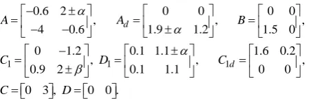
Example 1: First, consider an uncertain 2-D continuous system ( ) with the following parameters:
0.6 2 , 4 0.6 A
0 0
, 1.9 1.2 d
A
0 0 , 1.5 0 B
1
0 1.2 , 0.9 2 C
1
0.1 1.1 , 0.1 1.1 D
1
1.6 0.2 ,
0 0
d
C
0 3 ,
C D 0 0 .
with and uncertain parameters, bounded as follows : 1.2 1.2
and 1.8 1.8, which gives a four-vertices polytopic system.
[image:8.595.56.284.101.176.2]To design a 2-D filter for this system, we apply Theorem 2, first with g = 0, (quadratic filtering), the LMIs are infeasible. Then, for g = 1 (linearly parameter-dependent approach), we get =27.0765, whereas for g = 2, we obtain a better noise attenuation level: =20.0570. The number of LMIs and the number of scalar variables are compared in Table 1.
Table 1
g K L Time
0 1 2 3
Infeasible 27.0765 20.0570 20.0570
17 47 107 207
32 74 144 249
1.154 1.575 2.293 3.760 K is the number of scalar variables, L is the number of LMI rows involved in the optimization problem, and the computational times is given in seconds.
Example 2: Taking the same parameters in example 1 except replacing A by
0.6 4 4 0.6 A
and
2.6 2.6 1.8 1.8
first for g = 0, (quadratic filtering), the LMIs are infeasible. Then, for g = 1 (linearly parameter-dependent approach), we get = 43.0885, whereas for g = 2, we obtain a better noise attenuation level: = 21.3200.
[image:8.595.50.282.544.617.2]The number of LMIs and the number of scalar variables are compared in the following Table 2.
Table 2
g K L Time
0 1 2 3
Infeasible 43.0885 21.3200 21.3200
17 47 107 207
32 74 144 249
1.154 1.575 2.293 3.760 K is the number of scalar variables, L is the number of LMI rows involved in the optimization problem, and the computational times is given in seconds.
5.
CONCLUSIONS
This paper has studied the robust H filtering problem for 2-D continuous systems described by Roesser state-space models with state delays and uncertainty of polytopic type. A design methodology has been proposed based on using homogeneous polynomially parameter-dependent matrices of arbitrary degree: with the increasing degree, the obtained H filter design is less conservative. Numerical examples
efficient for the design of parameter-dependent filters for this class of systems.
6.
ACKNOWLEDGMENTS
This work is funded by A ECI A/030426/10 and MiCInn DPI2010-21589-c05 projects.
7.
REFERENCES
[1] M. Allouche, M. Souissi, M. Chaabane, D. Mehdi and F. Tadeo, "Takagi-Sugeno Fuzzy Observer Design for Induction Motors with Immeasurable Decision Variables: State Estimation and Sensor Fault Detection,"
International Journal of Computer Applications, vol. 23 No. 4, pp. 44-51, 2011.
[2] A. A. Babu, R. Yellasiri and N. and P. Hegde. "Robust Speech Processing in EW Environment." International Journal of Computer Applications, vol. 38, No. 11, pp. 46-50, 2012.
[3] A. Mehrotra, K. K. Singh and M.J. Nigam, "A Novel Algorithm for Impulse Noise Removal and Edge Detection," International Journal of Computer Applications, vol. 38, No. 7, pp. 30-34, 2012.
[4] R. N. Banavar and J. L. Speyer, “A linear-quadratic game approach to estimation and smoothing,” in Proc. 1991 American Control Conference, Boston, MA, June 1991, pp. 2818-2822.
[5] M. Chau, A. Luo and V. Chau. "PID-Fuzzy Control Method with Time Delay Compensation for Hybrid Active Power Filter with Injection Circuit," International Journal of Computer Applications, vol. 36, no. 7, pp. 15-21, 2011.
[6] F. F. G. Areed, M. S. El-Kasassy and Kh. A. Mahmoud,
"Design of Neuro-Fuzzy Controller for a Rotary Dryer,"
International Journal of Computer Applications, vol. 37, no. 5, pp. 34-41, 2012.
[7] C. El-Kasri, A. Hmamed, T. Alvarez and F. Tadeo,
"Robust H Filtering of 2D Roesser Discrete Systems : A Polynomial Approach," Mathematical Problems in Engineering, vol. 2012, pp. 1-15, 2012.
[8] C. W. Chen, J. S. H. Tsai, and L. S. Shieh, "Modeling and solution of two-dimensional input time-delay system," J. Franklin Inst., vol. 337, pp. 569-578, 2002. [9] C.E. De Sousa, L. Xie and Y. Wang, "H filtering for a
class of uncertain nonlinear systems," Systems and Control Letters, vol. 20, pp. 419 - 426, 1993.
[10] C. Du and L. Xie, " H Cntrol and Filtering of two-Dimensional Systems," Heidelberg, Germany, Springer Verlag, 2002.
[11]M. Fu, "Interpolation approach to H optimal estimation and its interconnection to loop transfer recovery," Systems and Control Letters, vol. 17, pp. 29 - 36, 1991.
[12] K. Galkowski, "LMI based stability analysis for 2D continuous systems," in Proc. 9th IEEE int. Conf. Electron., Circuits Syst., Dubrovnik, Croatia, pp. 923-926, Sep. 2002.
delayed systems," IEEE Trans. Signal Process., vol.52, no. 6, pp. 1631-1640, Jun. 2004.
[14] H. Gao and C. Wang, "Robust L2L filtering for uncertain systems with multiple time-varying state delays," IEEE Trans. Circuits Syst. I, vol. 50, no. 4, pp. 594-599, Apr. 2003.
[15] E. Gershon, D.J.N. Limebeer, U. Shaked and I. Yaesh, "Robust H filtering of stationery continuous-times linear systems with stochastic uncertainties", IEEE Trans. automat. Control, Vol. 46, pp. 1788 - 1793, 2001. [16] A. Hmamed, M. Alfidi, A. Benzaouia, and F. Tadeo,
"LMI Conditions for Robust Stability of 2D Linear Discrete-Time Systems", Mathematical Problems in Engineering, Article ID 356124, 11 pages, 2008. [17]A. Hmamed, M. Alfidi, A. Benzaouia, and F. Tadeo,
"Robust stabilization under linear fractional parametric uncertainties of two-Dimensional system wiyh Roesser models," Int. J. of Sciences and Techniques of Automatic Control and Computer Engineering, Special Issue, pp. 336-348, Dec 2007.
[18] C. El-Kasri, A. Hmamed, T. Alvarez, F. Tadeo, "Robust H filtering for uncertain 2-D continuous systems, based on a polynomially parameter-dependent Lyapunov function," 7th International Workshop on Multidimensional (nD) Systems (nDs), Sept. 2011. [19] A. Hmamed, F. Mesquine, F. Tadeo, M. Benhayoun and
A. Benzaouia,"Stabilization of 2D saturated systems by state feedback control," Multidim Syst and Sign Process, vol.21, no.3, pp. 277-292, Apr 2010.
[20] J. Huang, G. Lu, and X. Zou, "Existence of traveling wave fronts of delayed lattice differential equations," J. Math. Anal. Appl., vol. 298, pp. 538-558, 2004.
[21] S.H. Jiu and J.B. Park, "Robust H filtering for polytopic uncertain systems via convex optimization," Proc. Inst. Elect. Eng. Control Theory Appl, vol. 148, pp: 55 - 59, 2001.
[22] M. S. Mahmoud, Robust Control and Filtering for Time-Delay Systems. New York : Marcel Dekker, 2000. [23] N.E. Mastorakis and M. Swamy, "A new method for
computing the stability margin of two dimensional continuous systems," IEEE Trans. Circuits and Systems I, vol. 49, pp. 869 - 872, 2002.
[24] K.M. Nagpal, P.P. Khargonekov, "Filtering and smoothing in an H setting", IEEE Trans. Automat. Control, vol. 36, pp. 152 - 166, 1991.
[25] R. C. L. F.Oliveira, P. L. D. Peres. LMI Conditions for Robust Stability Analysis Based on Polynomially Parameter dependent Lyapunov Functions. Systems and Control Letters, vol. 55, no. 1, pp. 52-61, 2006.
[26] R. M. Palhares, C. E. D. Souza, and P. L. D. Peres, "Robust H filtering for uncertain discrete-time state-delayed systems," IEEE Trans. Signal Process., vol. 49, no. 8, pp. 1696-1703, Aug. 2001.
[27] P.G. Park, T. Keileth, "H via convex optimization", Int. J. Control, vol. 66, pp. 15 - 22, 1997.
[28] W. Paszke, J. Lam, K. Galkowski, S. Xu, and Z. Lin, "Robust stability and stabilization of 2-D discrete state-delayed systems," Syst. Control Lett., vol. 51, pp. 277-291, 2004.
[29] W. Paszke, J. Lam, K. Galkowski, S. Xu, and E. Rogers, "H control of 2-D linear state-delayed systems," presented at the 4th IFAC Workshop Time-Delay Systems, Rocquencourt, France, Sep. 8-10, 2003. [30] M. S. Pickarski, "Algebraic characterization of matrices
whose multivariable characteristic polynomial is Hermitian", in Proc. Int. Symp. Operator Theory, Lubbock, TX, 1977, pp. 126-126.
[31] E. Rogers, K. Galkowski, and D. H. Owens, "Delay differential control theory applied to differential linear repetitive processes," presented at the Amer. Control Conf., Anchorage, AK, May 2002.
[32] U. Shaked, "H minimum error state estimation of linear stationary processes", IEEE Trans. Aut. Control, vol. 35, pp: 554 - 558, 1990.
[33] H.D. Tuan, P. Apkarian, T.Q. Nguyen and T. Narikiys, "Robust mixed H2 H filtering of 2-D systems", IEEE Trans. Singal Process, vol. 50, pp. 1759 - 1771, 2002. [34] L. Xie, C. Du, C. Zhang and Y.C. Soh, "H2 H
deconvolution filtering of 2-D digital systems", IEEE Trans. Signal Process, vol. 50, pp : 2319 - 2332, 2003. [35] S. Xu,J. Lam,Y. Zou, Z. Lin, and W. Paszke, "Robust
H Filtering for Uncertain 2-D Continuous Systems" IEEE Transactions on Signal Processing, vol. 53, pp. 1731-1738, 2005.
[36] S. Xu and P. Van Dooren, "Robust H filtering for a class of nonlinear systems with state delay and parameter uncertainty", Int. J. Control, vol. 75, pp. 766 - 774, 2002. [37] I. Yaesh and U. Shaked, "Game theory approach to
optimal linear state estimation and its relation to the minimum H-norm estimation", IEEE Trans. Automat. Control, vol. 37, pp. 828 - 831, 1992.
[38] I. Yaesh and U. Shaked, "Game theory approach to optimal linear estimation in the minimum H norm sense," in Proc. 28th IEEE Conf. Decision Control, Tampa, FL, Dec. 1989, pp. 421-425.
[39] B. G. Zhang and C. J. Tian, "Oscillation criteria of a class of partial difference equations with delays," Comput. Math. with Appl., vol. 48, pp. 291-303, 2004. [40] B. G. Zhang and C. J. Tian, "Stability criteria for a class