A Highly Effective Adaptive Switching Mean Filter
Algorithm for Salt and Pepper Noise Removal
Aly Meligy
Mathematics & ComputerScience dept .Faculty of science. Menoufiya University
Hani M. Ibrahem
Mathematics & ComputerScience dept .Faculty of science. Menoufiya University
Sahar Shoman
Mathematics & ComputerScience dept .Faculty of science. Menoufiya University
ABSTRACT
This paper presents an efficient three-stage adaptive switching mean filter to remove salt-and-pepper impulse noise from highly corrupted images. Firstly, the noise detection stage is to detect pixels as “noise pixels” and “noise-free pixels”. The detected “noise pixels” will then be subjected to the second stage which is the noise cancellation, while “noise-free pixels” are retained and left unchanged. The method adaptively changes the size of the filtering window based on the number of the “noise-free pixels” in the neighborhood. For the filtering, only “noise-free pixels” in the window are considered to find the mean value. If this value is not available in the maximum window size, the last processed pixel value is used as the replacement. In the third stage, this algorithm utilizes previously processed neighboring pixel values to get better image quality as the really processed noise pixel used as a noise –free pixel for the next noisy pixel processing. Experimental results clearly show that the proposed algorithm outperforms many of the existing methods in terms of visual quality and quantitative measures. The advantage of the proposed method is that it works well for high-density salt & pepper noise even up to a noise percentage of 95%.
General Terms
Image processing, Image filtering, Noise reduction.
Keywords
salt-and-pepper noise, mean filter, adaptive filter, switching filter
1.
INTRODUCTION
Images often get corrupted by impulse noise during the acquisition or transmission. An important type of impulsive noise is salt & pepper noise. In salt & pepper corrupted images, noisy pixels take either maximum or minimum value degrading the image quality. Removal of salt & pepper is an important pre-processing step because it can influence the subsequent phases in image processing such as segmentation, edge detection and recognition [1].
The Standard Median Filter (SMF) is one of the most widely used non-linear noise filtering techniques to remove this noise, due to its denoising capability and computational efficiency. The main drawback of (SMF) is that it processes all pixels in the image equally, including the “noise free pixels” .Thus, it is effective only for low noise densities and at high noise densities, it often exhibits blurring for large window sizes and insufficient noise suppression for small window sizes [2].Many variations and improvements of median filter have been introduced such as weighted median
filter [3], center weighted median filter[4] and recursive weighted median filter [5] .Anther type of the median based methods is the switching method, which is constructed from two stages. The first stage is to detect the “noise-pixels”. The second stage is to remove only the “noise-pixels” while the “noise-free pixels” are kept unchanged.
The common drawback among all of these filtering techniques is that the noisy pixels are replaced without taking into account local features such as the presence of edges and the noise level. Hence details of the images and edges are not recovered satisfactorily, especially when the noise level is high. So, adaptive median filter is improved in many literatures such as [6] and [7].The classic adaptive median filter algorithm [7] aims to reduce noise density by expanding the window size .However, it has two drawbacks: (1) The original noisy pixel is kept unchanged when failing to find the median value in the maximum window size; (2) The noisy pixels are considered in the calculation of median operation. In this paper, an efficient adaptive switching mean filtering algorithm for salt and pepper noise removal is proposed. Switching mean filter framework is used in this algorithm in order to speed up the process and allow local details in the image to be preserved because only the noise pixels are filtered .Thus, it takes a decision whether the pixel under test is corrupted or not before applying the filtering which applied only to the detected “noise pixels “in the input image. This method adaptively changes the size of the filter based on the number of the “noise-free pixels” in the neighborhood. For the filtering, only “noise-free pixels” are considered for the finding of the average value of noisy pixel. This algorithm utilizes previously processed neighboring pixel values to get better image quality. The experimental results demonstrate that the proposed technique is effective for removing noise and preserving fine details than other existing denoising methods .The rest of this paper is organized as follows , in section 2 a related work is introduced. The proposed algorithm is presented in section 3. The implementation result and comparison are provided in section 4. Finally, conclusion is presented in section 5.
2.
RELATED WORK
neighborhood. For the filtering, only “noise-free pixels” are considered for the finding of the median value .For each noisy pixel, the number of “noise-free pixels” ,contained in the filtering window, must be larger than or equal to eight pixels .If this condition is not met ,the size of the filter will be increased by two .This procedure is repeated until the condition is met then the central noisy pixel is replaced with the median value. Further, Srinivasan and Ebenezer [9] have proposed a new fast and efficient decision-based algorithm (DBA) for removal of high-density impulse noises .This algorithm is proposed for restoration of images that are highly corrupted by impulse noise. It processes the corrupted image by first detecting the impulse noise. The detection of noisy and noise-free pixels is decided by checking whether the value of a processed pixel element lies between the maximum and minimum values that occur inside the selected window. This is because the impulse noise pixels can take the maximum and minimum values in the dynamic range (0, 255). If the value of the pixel processed is within this range, then it is an uncorrupted pixel and left unchanged. If the value does not lie within this range, then it is a noisy pixel and is replaced by the median value of the window or by its neighborhood values. For obtaining the new value of the processed pixel, the method depend on the median, maximum, and minimum pixels values within the selected window. Pei-Yin Chen and Chih-Yuan Lien [10] have proposed an efficient edge-preserving algorithm for removal of salt-and-pepper noise from corrupted images. It can preserve edges very well while removing impulse noise. This algorithm is composed of two components: efficient impulse detector and edge preserving filter. The former determines which pixels are corrupted by fixed-valued impulse noise. The latter reconstructs the noisy pixels by observing the spatial correlation and preserving the edges efficiently. For each noisy pixel, the image filter detects edges in six directions first and estimates the intensity value of the pixel accordingly. In addition, S. Esakkirajan et.al. [11] have proposed a modified decision based unsymmetrical trimmed median filter algorithm for the restoration of gray scale, and color images that are highly corrupted by salt and pepper noise. This algorithm replaces the noisy pixel by trimmed median value when other pixel values, 0’s and 255’s are present in the selected window and when all the pixel values are 0’s
and
255’s then the noise pixel is replaced by mean value of all the elements present in the selected window. Xiao Kang et.al. [12] have proposed a novel adaptive switching median filter for laser image based on local salt and pepper noise density .This algorithm for Laser image which often mixes with salt and pepper noise when obtained and transmitted by image sensor. Pixel points are divided into salt and pepper noise points and signal points according to two level detection mechanisms firstly, then, local salt and pepper noise density is introduced here to determined filter window of every noise point, only noise points are filtered by different size window adaptively whereas signal points are kept unprocessed finally.3.
THE PROPOSED METHOD
The proposed adaptive switching mean filtering algorithm includes three stages: (1) Noise Detection, (2) Noise Cancellation, (3) Noisy Image and Detection Map Update.
3.1
Noise Detection
In this method, switching mean filter framework is used in order to speed up the process because only the noise pixels are
In this stage, the processing pixel is checked whether it is noisy or noisy free. That is, if the processing pixel lies between maximum and minimum gray level values then it is noise free pixel, it is left unchanged. If the processing pixel takes the maximum or minimum gray level then it is noisy pixel which is processed by the filtering operation.
Assuming that the two intensities
j i
P, that present “salt and
pepper noise” are the maximum (K) and the minimum (0) values of the image’s dynamic range. Considering this
assumption, a binary value is assigned to each elements
D
di,j of the detection map D. The detection map is
computed from the noisy image as follows:
The entries of “1” and “0” in the detection map D represent the noisy and the noise-free pixels, respectively.
3.2
Noise Cancellation
This stage is applied only to the detected noise pixels in the input image. Adaptive filter framework is used in order to enable the flexibility of the filter to change its size accordingly based on the number of the “noise-free pixels” in the neighborhood.
For each detected ‘noise pixel’ Pi,j ,the size of the filtering
window (W×W) is initialized to 3×3 and an array R with length LR is populated with noise-free-pixels contained in the window. The length of array, depending upon the noise density within the window, varies from zero to eight. The minimum length zero shows all pixels in the window are noisy, whereas the maximum length eight indicates all eight pixels are noise-free. To estimate the value of noisy pixel, we emphasize noise-free pixels and a constraint of minimum three noise-free pixels in the array R (i.e. LR≥3). If this
condition is satisfied, then the central noisy pixel is replaced with the mean of R as
If the current filtering window does not have a minimum
number of three “noise-free pixels” (i.e. LR <3) and the filter
size is less than the maximum size WMax=7, then the filtering
window will be expanded by two in its size (W=W+2). This procedure is repeated until the criterion of (LR≥3) is met. We
prefer to use W=7 as a maximum filter size because the larger size window may not be too efficient and effective and the correlation between pixels decreases as pixels are separated apart. Moreover, the larger window may also remove the edges and fine image details.
Considering this possibility, the search for “noise-free pixels” is halted when the detected “noise-free pixels” are less than three (LR<3) and at the same time, the filtering window has
reached a size of 7×7. In this case, we replace the central noisy pixel with the last processed pixel. If the current W×W window doesn’t meet the condition and its size can’t be increased by two as it reached to its maximum size especially the boundary pixels, in this exception we also replace the
(1) , 0 0 P P if 1, j i, j i, , otherwise K dij
(2)
)
(
R
mean
3.3
Noisy Image and Detection Map
Update:
If the noisy pixel is replaced with the average estimated, then the detection map is also updated by changing the entries at the corresponding location in the detection map from “1” to “0” as
In this stage, the algorithm utilizes previously processed neighboring pixel values to get better image quality as the really processed noise pixel used as a noise –free pixel for the next noisy pixel processing.
The proposed method is summarized by the following algorithm, For each pixel location (i,j) with di,j=1 (i.e noise pixel) :
Step 1: Initialize the filtering window size to W=3, where WMax = 7.
Step 2: Assign the number of “noise –free pixels” contained in the filtering window to L.
Step 3: If L<3, go to step 6.
Step4: Calculate the average (Avg) based on the “noise-free pixels” contained in W×W window.
Step5: Replace the central noisy pixel with the average value and go to step 7.
Step6: If W ≤ WMax , then the filtering window will be
increased by two ( i.e. W =W+2) and return to step 2 ,else replace the central pixel with the last processed pixel in the neighborhood.
Step 7: Update the input noisy image and the detection map D to use the processed pixel as a noise-free pixel for the next processed pixel.
In the proposed algorithm, the filter performs denoising iteratively for each noise pixel until all the corrupted pixels in the noisy image are eliminated (see figure 1).
Fig 1: The flowchart of the proposed algorithm
Yes
No
Read The processed pixel P(i,j)
0<P(i,j)>255 Keep P(i,j) unchanged
Select a 2D W×W window with center element P(i,j) and Initialize the window size to W=3
Assign the number of “ noise –free pixels” in the window to L
L>=3 W ≤ WMax
, W
Max=7
Is W can expand?
Increase W by two,
W =W+2
Calculate the average value(Avg) based on the “noise-free pixels” contained in W×W window
Replace P(i,j) with the last processed pixel
Replace P(i,j) with the average value (Avg)
Update the input noisy image by replacing the central noisy pixel with the new value
Yes
Yes Yes
No
No
No
(3)
,
3
1
,
0
, ,
,
otherwise
d
L
d
if
d
j i
R j
i j
4.
RESULTS AND DISSUCTION
In the paper, several experiments are carried out to analyze the performance of the proposed scheme with dynamic range of values (0, 255). The simulation results of four standard images of Lena, Baboon, Boat, and Bridge are reported. These images of size 512×512 are corrupted with varying level of noise density (ND) from 10 % to 95 % using the salt-and-pepper noise. The simulation results obtained from the proposed scheme are compared with other salt-and-pepper noise filtering algorithms: Standard Median Filter (SMF) , Decision-Based Algorithm( DBA) [9],Simple Adaptive Median Filter (SAMF) [8], and Modified Decision Based Unsymmetric Trimmed Median Filter (MDFUTMF) [11].We used the peak signal-to-noise ratio (PSNR) measure as a quantative evaluation to assess quality of the restored image and to compare the results quantitatively with previous filtering algorithms. The PSNR measure is defined as:
Where Xi,j is the original noise-free image, Gi,j is the restored
image, MSE is the mean square error and M×N indicates the size of pixels of the original and the restored images .The PSNR value of the proposed algorithm is compared against the existing algorithms by varying the noise density from 10% to 95% (see Table 1). It is observed that our proposed algorithm (PA) provided the best PSNR at high noise densities. A plot of PSNR against noise densities for Lena , Baboon, Boat ,and Bridge images are shown (see figure 2) and the PSNR curves demonstrate that the Proposed Algorithm (PA) is the best in performance. The qualitative analysis of the proposed algorithm at different noise densities for Lena, Baboon and Boat images are shown respectively (see Figure 3, 4 and 5). It shows that the proposed algorithm is capable of removing salt-and-pepper noise more effectively, while preserving the fine image details and edges.
[image:4.595.358.513.73.367.2]
Fig 2 . Comparison graph of PSNR at different noise densities for (a) Lena image, (b) Baboon image, (c) Boat
image, (d) Bridge image
5.
CONCLUSION
This paper presents an efficient technique to remove salt and pepper impulse noise from highly corrupted images. It is actually a hybrid of the adaptive filter with the switching filter based on the arithmetic mean operation. The advantages of this method are that it solves the drawbacks of the classic adaptive median filter algorithm. In addition, it utilizes previously processed neighboring pixel values to get better image quality .further, it does not need a threshold parameter and the training stage is not required. The performance of the algorithm has been tested at different of noise densities. Even at high noise density levels the proposed algorithm gives better results in comparison with other existing algorithms.
6.
REFERENCES
[1] Wei Li, Yanxia Sun and Shengjian Chen ,“A New Algorithm for Removal of High-density Salt and Pepper Noises,”, IEEE 2009.
[2] I. Pitas and A. N. Venetsanopoulos,” Nonlinear Digital Filters Principles and Applications,” Norwell, MA: Kluwer, 1990.
[3] Astola J and Kuosmanen P, “Fundamentals of Nonlinear Digital Filtering” Boca Raton , ” FL: CRC, 1997. [4] Ko S J and Lee Y H, “Center weighted median filters and
their applications to image enhancement,” IEEE Transactions on Circuits and Systems, vol. 38, 1991, pp 984-993.
[5] Arce G and Paredes J, “Recursive Weighted Median (5) ) ( 1 (4) ) 255 ( log 10 2 , 1 1 , 2 10 j i M i N j j i G X N M MSE MSE PSNR
0 5 10 15 20 25 30 35 40 45 PS N R SMF DBA SAMF MDBUTMF PA 0 5 10 15 20 25 30 35 40 4510 20 30 40 50 60 70 80 90 95 noise ratio PS N R SMF DBA SAMF MDBUTMF PA (a
)
0 5 10 15 20 25 30 35 40 4510 20 30 40 50 60 70 80 90 95 noise ratio PS N R SMF DBA SAMF MDBUTMF PA (c
)
0 5 10 15 20 25 30 35 4010 20 30 40 50 60 70 80 90 95
[6] Raymond H. Chan, Chung-Wa Ho, and Mila Nikolova, “Salt-and pepper noise removal by median-type noise detectors and detail preserving regularization”, IEEE Trans. Image Processing, vol. 14,no. 10, pp. 1479-1485, October 2005.
[7] H. Hwang and R. A. Haddad, “Adaptive median filters: New algorithms and results”, IEEE Trans. Image Processing, vol. 4, no. 4, pp. 499-502, April 1995. [8] Haidi Ibrahim, Nicholas Sia Pik Kong and Theam Foo
Ng,” Simple Adaptive Median Filter for the Removal of Impulse Noise from Highly Corrupted Images,” IEEE Transactions on Consumer Electronics, Vol. 54, No. 4, November 2008.
[9] K. S. Srinivasan and D. Ebenezer,” A New Fast and Efficient Decision-Based Algorithm for Removal of High-Density Impulse Noises,” IEEE SIGNAL
PROCESSING LETTERS, VOL. 14, NO. 3, MARCH 2007.
[10]Pei-Yin Chen and Chih-Yuan Lien, ” An Efficient Edge-Preserving Algorithm for Removal of Salt-and-Pepper Noise,”IEEE SIGNAL PROCESSING LETTERS, VOL. 15, 2008.
[11]S. Esakkirajan and T. Veerakumar et.al. ,” Removal of High Density Salt and Pepper Noise Through Modified Decision Based Unsymmetric Trimmed Median Filter,” IEEE SIGNAL PROCESSING LETTERS, VOL. 18, NO. 5, MAY 2011.
(a)
(b)
(c)
Fig 3. (a) Original 'Lena' image , (b) 'Lena' image corrupted with 30% ,(c) Output of the proposed method .
(a)
(b)
(c)
Fig 4. (a) Original 'Baboon' image,(b) 'Baboon' image corrupted with 50% , (c) Output of the proposed method
(a)
(b)
(c)
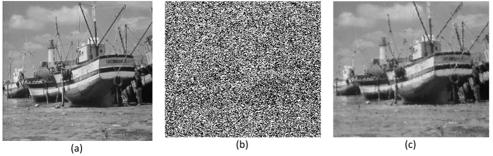
Fig 5. (a) Original 'Boat' image , (b) 'Boat' image corrupted with 80%, (c) Output of the proposed method
[image:6.595.55.539.68.228.2] [image:6.595.61.540.265.434.2] [image:6.595.53.543.472.627.2]Table 1: Comparison of PSNR values of different algorithms for Lena , Baboon, Boat , and Bridge images respectively
Lena Image
10% 20% 30% 40% 50% 60% 70% 80% 90% 95%
SMF(3×3) 33.9085 29.8645 23.7039 19.2248 15.2628 12.4080 10.0528 8.1563 6.6618 6.0190
DBA[9] 36.8199 33.9044 31.7456 28.7360 25.2938 21.9672 18.5844 15.0147 11.5929 9.6391
SAMF[8] 36.9998 32.3841 30.3480 28.8118 27.5963 26.0609 24.5417 22.5338 20.0325 18.1604
MDBUTMF [11] 42.7136 38.9992 36.5897 34.4640 32.1538 29.0257 24.6871 20.2110 15.9809 13.9076
PA 42.6193 39.2878 37.0283 35.2349 33.5170 31.6340 29.6914 27.3335 23.9264 21.1758
Baboon Image
10% 20% 30% 40% 50% 60% 70% 80% 90% 95%
SMF(3×3) 29.0304 26.9441 22.8935 18.7009 15.3300 12.4360 10.1332 8.3259 6.8122 6.1895
DBA[9] 36.8536 32.9135 29.9838 27.3456 24.1648 21.0440 17.8447 14.8783 11.5854 9.6895
SAMF[8] 33.7263 29.7970 27.4912 26.0124 24.9142 23.4256 21.9704 20.4616 18.6262 17.1973
MDBUTMF [11] 37.9596 34.4987 32.2676 30.3322 28.6624 26.4979 23.7418 20.2399 16.4650 14.6120
PA 38.3650 34.9011 32.5624 30.7441 28.9354 27.2518 25.4844 23.6458 21.5895 20.2653
Boat Image
10% 20% 30% 40% 50% 60% 70% 80% 90% 95%
SMF(3×3) 29.8434 27.4584 22.9733 18.8340 15.2372 12.3124 10.0013 8.1886 6.6741 6.0641
DBA[9] 37.4227 33.4271 30.6414 27.8768 24.8093 21.4992 18.2477 14.7737 11.5432 9.5521
SAMF[8] 35.2379 31.0923 29.1111 27.3610 26.0618 24.7122 23.0723 21.4012 19.2694 17.5934
MDBUTMF [11] 38.8632 35.2889 32.9842 31.1049 29.2432 26.7922 23.7151 19.8872 15.9324 13.9802
PA 38.4782 35.2436 33.1749 31.4639 29.9930 28.4434 26.7038 24.5981 21.8175 19.6119
Bridge Image
10% 20% 30% 40% 50% 60% 70% 80% 90% 95%
SMF(3×3) 26.1467 24.6778 21.7219 18.0625 14.7791 11.9923 9.7422 7.9266 6.4196 5.8246
DBA[9] 28.7159 26.2283 24.8345 23.6061 21.6307 19.5556 17.0765 14.0652 11.0497 9.1878
SAMF[8] 31.7723 28.4675 26.2552 24.8321 23.6480 22.4487 21.0629 19.7286 17.9016 16.3522
MDBUTMF [11] 34.2869 30.9936 28.9683 27.3740 25.8155 23.9065 21.4947 18.3041 14.6965 12.9211