Excess sensitivity of consumption using micro data in the UK

Munich Personal RePEc Archive

Excess sensitivity of consumption using

micro data in the UK

Yu, Ge

2005

EXCESS SENSITIVITY OF CONSUMPTION

USING MICRO DATA IN THE UK

1 INTRODUCTION

The arguments over the Permanent Income Hypothesis (PIH) and the rational

expectations extension of it (REPIH), concerning suggestions of excess sensitivity of

consumption, have been continued for decades without an explicit solution. This is

because there have been no conclusive findings in empirical studies. Most empirical

results show confidence in supporting one or rejecting the other. This vagueness has

significant and negative consequences for understanding the consumption/savings

processes of households and for improving our knowledge of economic trends and

stabilization from a policy perspective.

In the literature, many researchers have carried out investigations to test the validity of

assumptions such as hyperbolic discount rates1, binge augmented consumption, habit

persistence, and the excess sensitivity of consumption to income. However, only a few

empirical papers have investigated the impact of individual subjective information on

economic outcomes.

The methodology developed by Souleles (2001) to test for excess sensitivity with respect

to household data has a deep intuitive appeal. Rather than testing excess sensitivity using

aggregate data, Souleles used US household-level data from the Michigan Index of

Consumer Sentiment. He found that consumer sentiments were useful in forecasting

future consumption, even after controlling for lagged consumption and macro variables

such as stock prices. Furthermore, the systematic demographic components in forecast

errors were used to reject of the PIH. Melvin (2003) also examined the link between

subjective job loss expectations and the subsequent impact on household consumption

behavior behind the intuition suggested by Flavin (1981) and Campbell and Deaton

(1989).

In this paper, I follow Souleles (2001) and Melvin (2003) by using data derived from the

BHPS. This contains questions on the expected level and changes in a number of relevant

economic variables and British respondents’ uncertainty in making these predictions

covering the years 1991 until 2002. One of the main novelties of this thesis is that it uses

the financial situation validate in the BHPS to value the respondents’ well being instead

of the term ‘income’ popularly used in most papers. This is particularly interesting due to

the potential relationship between macro-economic shocks and individual psychological

well-being. Thus, while a narrow interpretation of financial situation is income, a broader

interpretation would take into account the values of any assets agents hold and the

incomes they currently received or expect to receive in the future. Most interesting, some

who experience an increase in current income may feel themselves worse off financially.

This is similar to the results in paper 5 in which respondents’ expectations decrease with

increasing real income. In other words, the idea of an agent’s financial situation or

satisfaction can potentially include many factors that are difficult to identify or value but

can significantly affect agents’ decision making behaviour in the real world. Furthermore,

Das and Van Soest (1996) argue that subjective answers reflect real rather than nominal

changes. Although the questions in the BHPS are not very well specified, it seems

reasonable to assume that respondents have the same broad concepts in mind when

answering questions on their financial outcomes and future expectations. In each wave of

the BHPS, agents answer questions on whether their actual financial situation has

changed in the past twelve months, and on whether they expect it to change over the next

twelve months. Both questions are answered on a three points scale2. In addition, the

following analysis breaks down the whole sample into various sub-samples to test for

excess sensitivity among each of these groups. It is hoped that these results can provide a

deeply insight into the divergence of sensitivity of each individual component to

consumption fluctuations.

2 RELATED STUDIES

Hall’s random walk hypothesis of consumption argues that if agents have rational

expectations (that is, if they are forward-looking) then current consumption should only

depend on consumption in the most recent period, and that not other variables will feature.

The implication of the REPIH is that if all past and predictable information is

incorporated in current consumption, no lagged information can provide additional

explanatory power in accounting for variations in future consumption. Thus, one way to

test the predictions of the REPIH is to examine whether consumption is sensitive to

anticipated changes in interested explanatory variables such as income. This approach has

been taken by Hall and Mishkin (1982), Altonji and Siow (1987), Attanasio and

Browning (1995) and Lusardi (1996) among others. As a means of testing the impact of

lagged variables on consumption, regression equations of the following from have been

introduced:

1 1

1 ( + ) +

+ = +

Δct βEt yt εt or Δct+1 =βEt(yt+1 −yt)+εt+1 (1)

Where y is household real income. If theoretical predictions of the permanent income

model and rational expectations are valid then H₀:β =0. In many studies (eg. Hall,

1978; Zeldes, 1989; Jappelli et al., 1998) the (log) level of income is used. Attanasio and

Weber (1993) used the growth in income. It is noted that the income term can be

considered as predictable income or income growth in t or t+1, using instruments dated

t-1 or earlier. The Euler equation is a period-to-period arbitrage condition and therefore does not take into account the effects of future constraints on current behavior. As such,

when estimating Euler equations using panel data. Chamberlain (1984) states that “a time

average of forecast errors over T periods should converge to zero as N →∞. But an average of forecast errors across N individuals surely need not converge to zero as

∞ →

N ; there may be common components in those errors, due to economy-wide innovations.” As a result, a set of time dummies are also included in equation (6.1) to

guard against this problem in many empirical studies3. Altug and Miller (1990) claim that

these dummies can be interpreted as the undiversified aggregate risk facing intertemporal

decisions under a complete market setting. Although the panel data (1991-2002)

employed in this thesis is longer than that used in some earlier studies, the time

dimension may still not be long enough. As a result, time dummies are included in the

regressors.

Flavin (1981) used the excess sensitivity tests to mount a powerful rejection of the

REPIH. Two ideas are developed in her work. One is that a stronger test for consumption

than the reduced-form consumption equation is provided. In addition, she attempts to

identify consumer’s reaction to both anticipated and unanticipated income shocks.

Flavin’s model mainly focuses on the role played by current income in providing new

information about future income. Under the permanent income hypothesis a rational

agent can use such information to upgrade his/her permanent income expectations. A

drawback of Flavin’s test is that both income and consumption processes need to be

modeled and the results which emerge from this are sensitive to the modeling

specifications that are used4.

Thus, a trended ARMA representation was used to model the time-series properties of the

income process and to specify agent’s expectations about their future levels of income.

Under assumption of an ARMA process for income, actual revisions in permanent

income can possibly be acquired from the contemporaneous observation of current

3

Zeldes (1989), Altongji and Siow (1987), and Runkle (1991)

income. This revision is given by the forecast error in the ARMA specification and such

an error represents unanticipated news associated with current observations of income5.

The magnitude of the revision would then depend on the parameters of the ARMA

representation of the income process. Together with this argument, one can ‘specify a

structural equation relating the change in consumption to the contemporaneous revision

in permanent income (modeled using the income innovation) and the change in current

income’. [pp.976]. As a result, it is possible to use Flavin’s model to explore the

determinants of change in consumption for inferring agents’ expectations.

Since the path of future income is uncertain, an individual must make his consumption

plans on the basis of some set of expectations about future income. Given the

expectations about future income held in period t, the individual’s permanent income can be expressed as

⎥ ⎦ ⎤ ⎢ ⎣ ⎡ + + =

∑

t E y

r A

r

y (2)

where is permanent income at time t; is their stock of assets at time t; r is the

constant real rate of interest; is their labor income at time t; and is the

expectations operator for expectations at time t.

p t

y A_t

t

y Et

Allowing for a stochastic, or transitory, component of consumption, the consumption

function for the representative individual becomes t, or

p t t y u

c = +

t k k t t k t

t E y u

r A

r

c _⎥+

⎦ ⎤ ⎢ ⎣ ⎡ + + =

∑

( (3)

5

where the error term ut denotes the transitory component of consumption.

Solving for c_t+1 in terms of c_t, subject to A_t+1 =(1+r)A_t + y_t −c_t, gives:

∑

1 ) ( ) (1 )

1 1 ( k t t k t t t k t

t E E y r u u

r r

c

c (4)

Consumption will evolve as random walks only if the transitory consumption term is

identically zero, u_t ≡0. So I can re-write

⎥ ⎥ ⎦ ⎤ ⎢ ⎢ ⎣ ⎡ − ⎟ ⎠ ⎞ ⎜ ⎝ ⎛ + + − ⎟ ⎠ ⎞ ⎜ ⎝ ⎛ + = − + = Δ

∑

∑

Consequently I use the above equation to understand how changes in expectations of

future income relate to consumption changes. Because the first term represents the

household’s expectations errors concerning current income, , while the second term

corresponds to the influence of changing expectations regarding future income ,

, changes in consumption between the two periods can be decomposed into these

two terms. A basic empirical implication of this model is that, even if the behavioral

marginal propensity to consume out of current income is zero, consumption should

respond to changes in current income because these innovations provide new information

about future income and therefore induce revisions in expected permanent income. In

other words, one alternative hypothesis is that expectations errors might not be classical

but rather contain systematic components correlated with the excess sensitivity regressor.

Chamberlain (1984) states that systematic expectations errors can be a potential problem

in estimating any rational expectations (or forward-looking) model in a short panel. For

instance, female respondents might, on average, have been optimistic about future over

the sample period, so that they increase their consumption due to their over-optimism or a

positive correlation between consumption and expectations would not be inconsistent

with the REPIH. The availability of the direct measures of respondents’ expectations

errors in the BHPS makes it possible to test this point directly.

The null hypothesis in Flavin’s paper is the permanent income hypothesis associated with

an autoregressive specification for the process governing labor income. In general, it also

can be specified as followed:

) )( ( ) 1 ( ₁ 0 τ α αη

ε T t _{t t t k t k}

k

k t

t

t r E E w y

c _{− + +}

− = − _{− +} + = = =

Δ

∑

t t

y L ε

φ( ) = (7)

where . Flavin also introduces the possibility of unanticipated capital

gains in the model, so surprises in non-labor income, , are allowed to be different

from zero. Strictly speaking, Flavin’s excess sensitivity hypothesis allows consumption to

respond to current and lagged changes in income by more or less than is required by the

permanent income theory. The extended version of Flavin’s model is as followed:

τ k t k t k

t w y

y₊ = ₊ + ₊

τ

y

t t

y

L μ ε

ξ( ) = + (8)

t t t

t L y u

c = + + Δ +

Δ γ θε β( )

where ξ( )=

∑

i i p i L

L β(L)=

∑

Flavin rearranges the AR(p) income process equation and substitutes the error term ε_t into the consumption equation for income variable. Hence, the first difference of

innovation in the income process in the unrestricted version of the model. The measures

of excess sensitivity of consumption to current income,β, provide an estimate of the

amount of additional response of consumption to the new information contained in

current income. In sum, according to the REPIH, consumption changes should not be

related to other variables except of the amount to income innovation provided by the

error term ε . Hence all the β coefficients, which represent the extend to which

consumption responds to previously predictable changes in income, should be zero.

In Flavin’s paper, she runs an eight-order auto-regression (p=8) for the labor income

process. The restriction β₀ =β₁ =...=β₇ =0 is imposed on the system to obtain a

constrained system that can be estimated. She then used data on non-durable goods

consumption from 1949(3) to 1979(1) and found that the likelihood ratio statistic for the

hypothesis 0β₀ =β₁ =...=β₇ = was 27.02 for . Hence the random

walk specification of Hall was rejected by Flavin. [pp. 999]. The estimates for the first

three sensitivity parameters are .335, .071 and .049. These results indicate a strong excess

sensitivity response of consumption to changes in current income. [pp. 1002] 96

. 21 ) 8 (

2 ₌

χ

However Mankiw and Shapiro (1985) and Deaton (1992) began to question the validity

of the stationary income process assumption, one of the main econometric techniques

used by Flavin, and discussed the actual form that modeling the income process should

take when such a process appears to be non-stationary. They also criticized the method

used by Flavin to account for the upward trending behaviour of income which dealt with

the non-stationary nature of the income process by fitting exponential time-trends to both

consumption and income, and by replacing consumption and income in the regressions

by their residuals. In particular, Mankiw and Shapiro argued that excess sensitivity is

induced by this detrending procedure, even if excess sensitivity is not present in the data.

(8) cannot provide much information for both sides of the consumption equation as each

are of a different order of integration6. The problems about making inferences about the

coefficients on lagged income using standard t and F-tests are essentially the same as the problems that occur in discerning the existence of a unit root in a univariate time series,

and the use of standard normal tables at usual significance levels results in over-rejection.

Deaton (1992) ran a Monte Carlo experiment7 to test this point and found that the

t-statistics for excess sensitivity on each of the income variables, and the test for excess sensitivity as a whole (an F-test), rejected more than the customary 5%8.

However Stock and West (1988) challenged Mankiw and Shapiro’s suggestion that

excess sensitivity was the result of bad econometric practice by using the concepts of

cointegration and error correction to provide a means of testing excess sensitivity:

t d t d

t t

t b bc b y b y u

c = ₀ + _{1 −1} + _{2 −1}+ _{3 −2} +

where yd is the same income measure used by Flavin. Now, if savings is defined as

t t d

t t

t b b b c b b y b s u

c = ₀ +( ₁ + ₃) ₋₁+( ₂ − ₃) ₋₁ + _{3 −1} + (9)

We would see that the savings variable plays the error correction role in this model if we

expect the coefficient of the lagged consumption variable (b₁ +b₃) to be close to one.

Sims, Stock and Watson (1990) show that in a regression of integrated variables of the

same order, standard asymptotic theory can be applied to parameters that can be written

as the coefficients of stationary variables. If consumption and disposable income are

cointegrated, then the last two variables of equation (9) are stationary. Hence, it is

6

To see this note that in (21) the income equation is already in reduced form, and to obtain the reduced form for consumption I only need to substitute the income equation into the consumption equation (see Deaton (1992) pp. 89).

7

Deaton himself recognizes that ‘the Monte Carlo results, although tailored to reflect the actual data, do not generate results that look like Flavin’s’. [pp. 94]

8

possible to make inferences about the excess sensitivity parameters and . Stock

and West also used Monte Carlo experiments to show that their technique worked and

found evidence in favor of excess sensitivity. Thus, according to Stock and West, the

problem with Flavin’s test procedure is that the imposition of a unit coefficient upon the

lagged consumption variable alters the asymptotic distributions of the estimates.

However once we correct for this problem, evidence for excess sensitivity still appears to

exist.

2

b b3

3 DATA

4 METHODOLOGY

In life cycle models of individual behaviour, future expectations play an important role.

As a result, it is believed that they may help in making forecast of individual behaviour in

consumption or saving. This has lead to an increasing interest in data on, and the

modelling of, expectations. The preceding discussion has clearly indicated that standard

theoretical predictions are prone to dismissals primarily depending on the information

sets the household faces. Any assumption on the homogeneity of preferences and

information sets the households face might lead to inefficient evaluations. To deal with

this shortcoming, Souleles (2001) came up with a simple but novel way of estimating

consumption patterns by exploring the response of different types of households over

time. In this paper, following on from Souleles (2001) and from Melvin (2003), direct

information on respondents’ future financial change expectations, which are different

from the standard approach9 of inferring expectations from panel data on outcomes that

leads to the assumption of rational expectations are used, to test for excess sensitivity.

In this analysis, the individual’s financial variables are used as a proxy of income to

explore the relationship between financial well-being and household consumption. To the

extend, the current income shock yt+1−Etyt+1 is taken the place of the financial

expectations errors. Financial expectations change is related to future income

expectations change, . The first part of this paper follows Souleles’ (2001)

method to test for the excess sensitivity of consumption to changes in financial

expectations. To do this Souleles added the lagged expectations variable Fisitx to a standard linearized Euler equation for consumption. Thus, for household i the change in consumption between period t+1 and t is specified as

k t t t E y

E₊ − ) ₊ ( 1

) 10 ,..., 1 (

1 , 1 , , 1

1

, = + + + =

Δc_it+ αtime_t+ βFisitx_it γW_it+ ε_it+ t (10)

Where Δc refers to changes in household nondurable consumption10; time includes a full set of year dummies (1992~2002), which controls for all aggregate (uniform) effects,

including seasonality, aggregate interest rates, and other macro variables which allow for

changes in the households financial situation from year to year; Fisitx denotes the expectations of financial situation change; while W controls for demographic characteristics such as changes in the number of adults and children11 in the household.

There are many possible sources of excess sensitivity, such as myopia and the existence

of liquidity constraints. As a result, the second stage of the analysis is to explore the

possible sources of excess sensitivity associated with the whole sample and with some

sub-samples of it. The analysis also distinguishes between anticipated changes in

financial situation that are negative (deteriorated financial situation changes) from those

that are positive (improved financial situation changes). This asymmetry between

10

Since many studies examine the change in log consumption, the results of the analysis using this alternative dependent variable are presented as well.

11

negative and positive resource changes is first discussed in Altonji and Siow (1987) and

recently analyzed by Shea (1995b;1995a). A simple extension of equation (6.10),

following Shea (1995b), provides a deeper insight into the evolution of the consumption

process given the following:

) 10 ,..., 1 (

1 , 1 , , 2 , 1 1 1

, = + + + + =

Δ − + _{+ +}

+

+ time Fisitx Fisitx W t

c_it α _t β _it β _it γ _it ε_it (11)

where β1 and β2 are dummy variables indicating and respectively.

This form allows us to test whether excess sensitivity can be explained by the following

reasons.

−

t i

Fisitx,

+

t i

Fisitx,

1. Rule-of-Thumb Consumers. There are consumers who are myopic. They are assumed to have a constant marginal propensity to consume out of current wealth

or income and therefore do not behave as predicted by the REPIH. As a result,

such consumers will be excessively sensitive to variables known in the

information set. However, rule-of-thumb consumers will respond to changes in

their financial resources regardless of whether these are expected to be an

improvement (a positive change) or a deterioration (a negative change). In other

words, if consumers are myopic, β₁ and β₂ should both be significantly

positive and of similar magnitudes.

2. Liquidity Constraints. Consumption models based on the presence of liquidity constraints predict a stronger (positive) response in consumption growth to

positive predicted financial resource growth than to negative financial resource

growth because liquidity constraints only preclude borrowing against future

expected financial source growth but do not inhibit saving ahead of future

expected financial resource reductions. Hence consumers can save and smooth

outcome would also be expected if forecast errors represent a transitory financial

situation shock as in buffer-stock saving models, such behaviour reflects

‘self-imposed’ liquidity constraints. Thus, if liquidity constraints were the main

cause for rejections of the REPIH, we should observe excess sensitivity only

when consumers expect increases in financial resource but are prohibited from

borrowing. In such a case β2 should be significant if a household head is

genuinely liquidity constrained, but β₁ should be insignificant.

3. Asymmetric Preferences. Another plausible explanation for the excess sensitivity to predicted changes in financial resource is that households do not have

time-separable preferences as assumed. If there is inertia in preferences, perhaps

due to the role of habit formation, households will only adjust their behavior

slowly. In the case of asymmetric preferences, β1 should be significant while

2

β should be insignificant. Carroll (1995) applied two dummy variables to test

the existence of an asymmetric response of consumption to positive and negative

shocks to permanent income by using information on union contracts to construct

a measure of expected income growth for each household. He found that the

response of consumption to negative income shocks were much higher than those

associated with positive income shocks. Likewise, Bowman et al. (1998) used a database derived from five countries (Canada, France, West Germany, Japan, and

the United Kingdom) to estimate the expected income growth and found

empirical support for an asymmetry in consumption behaviour. Bowman et al’s method for estimating the expected income growth was to regress actual income

In most cases, economists who assume that individuals do not make systematic errors

under the REPIH find that it works well using aggregate data. Because the BHPS

involves information on individuals’ financial well-being, this paper tests to see whether

individuals’ subjective financial well-being influences their consumption behaviour

(non-durable consumption). Next, this paper examines the overall distribution of

individual financial well-being and consumption with respect to various categorizations

of household types.

To carry out a further investigation of the failure of Hall’s random walk hypothesis, this

paper then returns to the residual, ε, which determines changes in consumption and

potentially includes many factors, such as measurement error or unobserved

heterogeneity in discount rates. According to Flavin (1981), Campbell and Deaton (1989),

and Melvin (2003), equation (6) can help to decompose ε into two components: the

change in consumption resulting from unexpected current financial changes; and any

revisions in expected future financial situations. Empirically, the following equation (12)

is used, which shows a direct relationship between financial expectations errors and

household consumption, to assess whether systematic heterogeneity in expectations errors

can lead to spurious inference more generally in forward-looking models.

) 10 ,..., 1 (

1 , 1 , 1 , 1

, 1

1

, = + + + Δ + + =

Δc_it+ αtime_t+ βFisitx_t ϕFisite_it+ φ Fisitx_it+ γW_it+ ε_it+ t (12)

Where Fisite denotes financial expectations errors and ΔFisitx denotes changes in

respondents’ financial expectations. For consistent estimates of β, the forecast errors

need to be uncorrelated with the excess sensitivity regressor Fisitx. With direct measures of expectations errors, we can test the implications of systematic heterogeneity in the

errors. Also, shocks to financial situation are considered to be among the most important

sources of the overall changes in consumption in ε . Under the alternative hypothesis

we would expect to find β =0 and ϕ >0, since the REPIH allows for consumption to

respond to the current financial shocks represented by Fisite. εi,t =μi +vi,t, where

i

μ captures the unobserved, time-invariant characteristics of the individual. It means that,

for all observations relating to a given individual, μ_i will have the same value,

reflecting their unchanging unobserved characteristics. For μi to be properly specified,

it must be orthogonal to the individual effects. are random errors. In this case

and the

it

v

) , 0 ( ~ ), , 0 (

~ 2 2

v it

i IID σ v IID σ

μ μ μi are independent of the . In other words,

the cross-sectional specific error term

it

v

i

μ must be uncorrelated with the errors of the

variables if this is to be modeled with other explained variables. However the later

assumption is unrealistic in the present context, as W includes demographical variables

that are correlated with, for example, any unobserved ability captured in μ_i . Furthermore, if this unobserved individual specific effect is also correlated with the

expectations errors, then the main coefficient of interest, β, will be biased. Panel data

allow us to overcome these potential problems of endogeneity by treating the unobserved

effect μ_i as random, and I estimate equations (11) and (12) using random effect models.

In the process of developing detailed simulation models we need to identify a proxy for

non-durable consumption while food and grocery expenditures are considered to be fairly

unresponsive to changes in purchasing power in aggregate data, that is, the consumption

of food is relatively inelastic to income, at the level of individual or household. We might

expect to observe significant changes in food and grocery expenditure when there are

noticeable changes in their financial circumstances and a reasonably strong relationship

between food expenditures and their financial well-being. All specifications have the

derived from the BHPS, I exploit cross-sectional variation by controlling for time effects

and investigate the source of any excess sensitivity by using a random effects model.

5 RESULTS AND ANALYSIS

5.1 Evaluating Excess Sensitivity

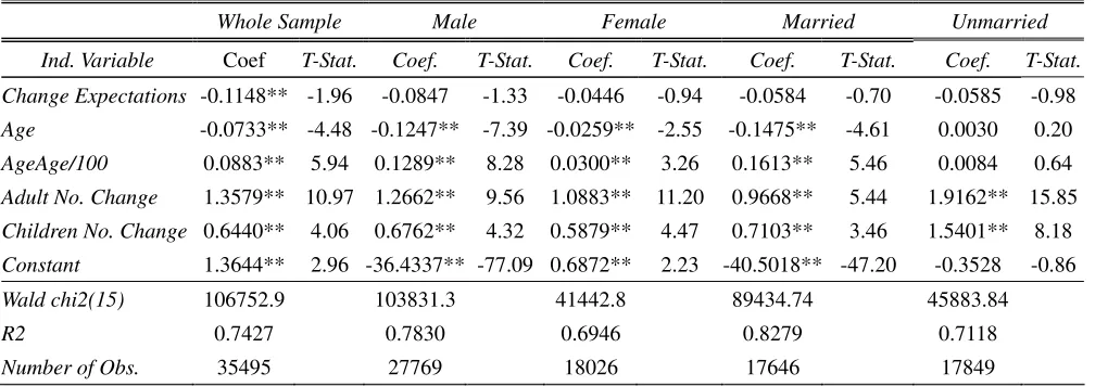
In terms of the excess sensitivity tests, there are two main findings. First, Table 1 in

Appendix provides robust estimates of the model parameters for the estimating equation

(10). If the REPIH holds, one would expect to find that the coefficient of financial well

being growth (β) would not be statistically different from zero. Instead the test reports a

significant β with a coefficient estimate of -0.1148 for nondurable consumption in the

whole sample. This clearly indicates that consumption fluctuated with anticipated

changes in financial well being and this amounts to a decisive rejection of the REPIH:

consumption is excessively sensitive to current financial well being changes, or, in other

words, it suggests that individuals fail to peg their consumption to expectation of their

permanent wealth.

Carroll (2001) explains the correlation between future expected resource growth and the

probability of excess sensitivity by arguing that such households are more likely to want

to borrow or because expected resource growth effectively raises the degree of

impatience. In addition, the information on financial expectations appears to help predict

consumption. The signs on β are negative in most sub-samples. Thus, in all cases,

better financial states are associated with less steep consumption profiles; that is, higher

expectations are associated with less saving. This outcome is both consistent with

precautionary motives for saving (Deaton, 1992; Carroll, 1992; Lusardi, 1998) as well as

with increases in expected future resources. While adding demographic variables into the

these variables act as important control variables. Thus age is employed as a significant

variable in the regressions. Age decreased consumption up to 41.5 and thereafter

increased it (because quadratic ax2 +bx+c turns over at

a b x

2

−

= , which for age

and age2 coefficient is ) 100 41.50 0883

. 0 2 ) 0733 . 0 (

(− − _× × ≈ ). Other demographic

terms also showed plausible signs. For example, there was a positive relationship

between consumption growth and family size or changes in the number of children.

Second, the evidence for excess sensitivity is statistically significant in only some

sub-samples. For example, with respect to household heads with highly educated level,

β(-0.1605) was statistically significant at the 5% level; however it was insignificant for

other groups in the education sub-sample. This suggests that high-educated agents fail to

smooth their consumption, but agents with comparatively lower education level smooth

consumption very effectively in the sense that they do not display excess sensitivity. In

the same vein, I can refer the employee, the self-employed, or higher degree holders as

the excess sensitivity groups. Among the other groups, agents’ expectations did not affect

their nondurable consumption. In other words, the REPIH could not be rejected for

results in these sub-groups.

5.2 Tests for Myopia and Liquidity Constraints

As was indicated earlier, deeper insights into the relationships between the excess

sensitivity of consumption and the dependence of consumption to financial situation

change can be obtained by extending equation (10) to equation (11). In addition, changes

in financial situation are divided into negative and positive parts to investigate whether

consumption changes are more sensitive to stochastic financial deteriorations or

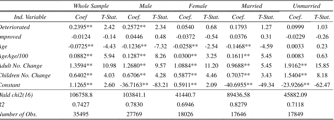
improvements. The estimated equation and results are presented in Table 2 in Appendix.

A similar set of instruments as in the previous case were used for these estimations. These

deterioration in their future financial situation. Conversely the coefficient of positive

financial well being growth is insignificant and ambiguous. The above exercise proves an

important point in that we can formally reject β1 =β2 =0 in favor of β1 >β2, a result

strikingly similar to that found by Shea (1995b).

Under predictable or expected financial well being changes, myopia would imply that

consumption fluctuates equally in response to both positive and negative financial

situation variations. Thus, if households are indeed myopic, they would be incapable of

pegging their consumption to their permanent income, in which case, consumption

should increase whenever their financial situation improves and decrease whenever their

financial situation deteriorates. Hence changes in consumption should be uniformly

related to changes in financial well being. This analysis finds that consumption is affected

only by negative financial well being growth. This does not conform to the situation of

myopic consumption behavior. One the other hand, if liquidity constraints exist, predicted

financial situation deterioration should make forward-looking individuals save more, and

thereby avoid a decline in their consumption. Therefore, consumption should be more

sensitive to predicted financial situation improvement than to financial situation

deterioration, due to existence of anticipatory savings. However, if financial well being

fluctuations are predictable, the above results are not indicative of either myopia or

liquidity constraints. And, the effect of anticipated financial well being fluctuations might

be quite different. Individuals, then, would be incapable of forecasting financial situation

deterioration. Thus it is plausible that an inability to borrow pulls consumption down with

deteriorated financial situation. Nevertheless, the failure of the REPIH is apparent from

the empirical results. However, the cause for this breakdown remains unclear in the

present analysis.

Consequently, asymmetric preferences appear to be the most important source of the

nonseparabilities in preferences, and I would focus on those that induce asymmetric

responses to positive and negative predicted financial resource changes. Such behavior

could arise if individuals weigh outcomes that are above and below a certainty equivalent,

or treat gains and losses differently.12 For example, if consumers with asymmetric

preferences (i.e., they are averse to negative changes) expect a negative income change in

t+1, they would gamble that the negative shock will not occur rather than revise

downward in expectation of the negative shock. A small reduction in and a large

negative change in can therefore translate into a large negative for a given

expected change in financial resources. In contrast, when consumers anticipate a future

but positive income change in period t, they will revise upward immediately just as

any expected utility maximizer would. This implies that

t

c

t

c

1 +

t

c Δct+1

t

c

1 +

Δct will be small in response

to the anticipated positive change in financial resources. In summary, I used equation (11)

to test three hypotheses and found that Asymmetric Preferences appears to be the most important source of excess sensitivity.

Turning to the results from sub-samples, the coefficients of anticipated financial well

being deterioration are significant in male, employee, and the highly educated groups in

line with the explanation of asymmetric preferences in the whole sample. However, the

coefficient of financial well being improvement is significant in self-employed group.

This result implies that liquidity constraints can be the source of excess sensitivity for the

self-employed respondents.

5.3 Detecting Excess Sensitivity in Systematic Heterogeneity

Another possibility, but one that has not previously received much scrutiny in the

12

literature, is systematic heterogeneity in expectations errors. This is especially likely to be a problem since both the financial situation variables and expectations errors were

found to be correlated with household’s demographic characteristics in paper five. These

findings suggest that even a long sample period and a full set of time dummies might not

be enough to ensure the orthogonality of the expectations errors with the financial

situation variables13. Furthermore, Flavin (1981) derives a model to identify the

consumers’ reaction to expectations errors and changes in expectations of their future

resources. The direct measures of households’ expectations errors found in the BHPS

make it possible to explore whether expectations errors play an important role in the

rejection of the REPIH. As a result the expectations errors were added into equation (10)

and equation (12) was used to consider whether systematic heterogeneity in expectations

errors was another source of excess sensitivity.

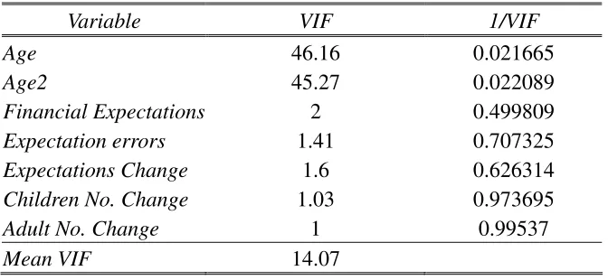
There is likely to be a multicollinearity problem if financial expectations changes are

correlated with expectations errors. In other words, even a long sample period and a full

set of time dummies might not be enough to ensure orthogonality of the expectations

errors with the financial expectations regressors. To test for multicollinearity each x was regressed on all of the other x variables. The 2

1−R from this regression was then used to see what fraction of the first x variable’s variance was independent of the other x

variables. The results from VIF (Variance Inflation Factor) Table 3 in Appendix give a

quick and straightforward check for multicollinearity. The 1/VIF column at right in a VIF

table gives the values equal to 1−R2 . It shows that 65.8% of the variance in

expectations errors’ was independent of age, age2, financial expectations, expectations change, change in number of adults, and change in number of children. Similarly, about 63.9% of the expectations change’s variance was independent of the other variables.

13

The VIF column in the center of the VIF table reflects the degree to which other

coefficients’ variances (and standard errors) are increased due to the inclusion of that

predictor. This shows that both expectations errors and expectations change have virtually no impact on the other variances. In sum, there is not substantial

multicollinearity in the regressions.

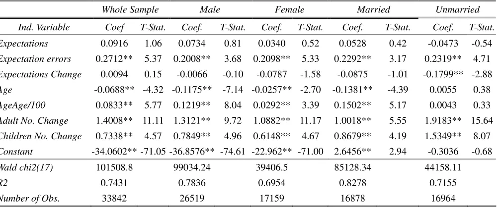
Table 4 in Appendix shows that the coefficients of ϕ on the expectations errors, Fisite,

are significant in the whole sample and nearly all of the sub-samples despite the inclusion

of the time dummies in the equation. It notes that the excess sensitivity regressor β

becomes insignificant in all groups, except for the self-employed and the respondents

with the secondary education level, when expectations errors and expectations changes

are controlled for. This means that some excess sensitivity persists among self-employed

and the secondary-educated respondents and is not due to heterogeneity in expectations

errors alone. However, for most respondents, some of the excess sensitivity appears to be

due to systematic heterogeneity in expectations errors. This suggests the possibility that

previous excess sensitivity tests might have made spurious inferences. Also, the resulting

coefficients of expectations errors in Table 4 are positive and marginally significant. In

other words, the more positive the expectations errors, the more pessimistic the

household is in regards to their financial situations and the larger is the magnitude by

which they would change their consumption. The coefficients φ of the changes in

expectations of future financial resources are not significant except for the unmarried and

the self-employed groups. The insignificance of the φcoefficients is consistent with the

assumption that changes in expectations of future financial resources are incorporated

into current consumption.

For more details about the response of consumption to expectations errors, I

over-pessimistic) from those that were negative (over-estimated/over-optimistic), and

denoted them by and , respectively. The equation now took the

form:

+ +1 ,t i

Fisite Fisitei−,t₊1

) 10 ,..., 1 ( 1 , 1 , 1 , 1 , 2 1 , 1 1 1

, = + + + + Δ + + =

Δ + _{+ + +}

+ −

+ +

+ time Fisitx Fisite Fisite Fisitx W t

cit α t β t ϕ it ϕ it φ it γ it εit

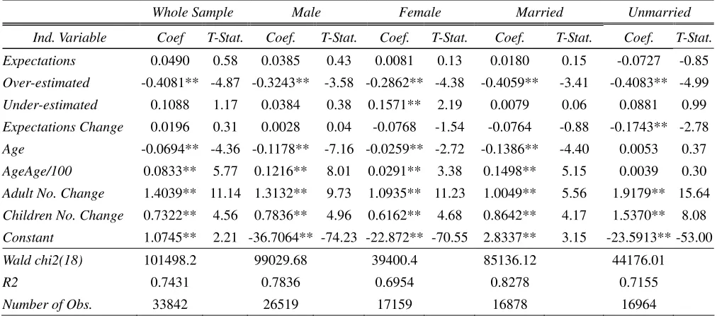
The results (Table 5) of splitting the expectations error term were again consistent with

the predicted result: positive expectations errors were positively correlated with

consumption but the relationship was insignificant except for higher-educated agents. In

addition, there was no significant differences in the consumption growth changes

between over-pessimistic agents and “smart” agents. This implies that agents refuse to

decrease their consumption level in when they are pessimistic about their future

financial source. will be small when their pessimistic expectations are proved to

wrong. In contrast, the coefficient for negative expectations errors (over-estimation) are

also of the correct sign and highly significant in most of the sub-groups. Thus consumers

who tend to be over-optimistic increase their consumption more than those that have

correct expectations of their future financial resources. It means that agents increase their

consumption as soon as they feel optimistic about their future financial resources. But, if

they are over optimistic, there would be a large increase in and a relatively less

increase or even a reduction in . This would lead to a negative consumption growth.

So, the results of splitting the expectations errors provide more evidence to support the

finding that asymmetric preferences are an important cause of excess sensitivity.

t

c

1 + Δct

t c 1 + t c 6 CONCLUSION

and has evaluated the model empirically with a household micro panel data set which

includes exhaustive information on consumption. The theoretical formulation presented

here is that of a benchmark consumption model following the main assumptions of the

REPIH. The primary focus of the discussion was to re-evaluate the excess sensitivity

puzzle of consumption behavior. Simple investigations on the BHPS data set, used for

empirical aspects of this thesis, revealed some interesting facts. What follows from this

empirical work is that consumption may be associated with other variables other than

financial wealth. In the introductory sections, I reviewed the work by Souleles (2001) and

Flavin (1981) which used US data sets. Their studies appear to be an excellent

benchmarks for formulating the analysis strategy: this empirically revisit the random

walk hypothesis of consumption using Souleles’s method; used the extensions presented

in Shea (1995b) to evaluate myopic consumption behavior and the existence of liquidity

constraints; and finally, a follow-up of the Flavin test of excess sensitivity was carried out

to investigate the role of expectations errors in explaining the excess sensitivity. While

this previous work used aggregate data to test the REPIH hypothesis, the present study

employed their methodology to investigate patterns from the BHPS data set.

The results clearly refute the predictions of the rational expectation extensions of the

PILCH. In the first regression (Table 1), the results indicate an excess sensitivity of

current consumption to one-period lagged financial well being.

In the next regressions, financial wealth growth was divided into positive and negative

parts. The results (Table 2) indicate that consumption fluctuations are significantly related

to financial wealth declines, but not related to financial wealth increases. However,

although the failure of the REPIH is substantiated from these results, they do not shed

light on whether it is myopia or liquidity constraints that are the main cause for this

failure. Ambiguity arises because if myopia exists, then consumption should fluctuate

and financial situation changes are predictable, individuals should be able to smooth their

consumption in cases of declines in financial wealth by saving beforehand, in forecast of

the future financial deterioration. If financial deterioration cannot be forecasted,

anticipatory saving is not plausible. In the presence of strict borrowing constraints,

households might face a fall in their consumption in such circumstances.

The third step tried to remove the ambiguity in understanding the cause for the

breakdown of the REPIH by turning whether the systematic heterogeneity in forecast

errors explains this breakdown. Previous studies, which lacked explicit measures of these

errors, have not been able to consider this hypothesis directly. Demographic components

of forecast errors were found to explain some of the excess sensitivity. Generally

speaking, since forecast errors are correlated with household demographic characteristics,

they will be correlated with many regressors of interest in forward-looking models,

suggesting that non-classical forecast errors are in practice a general and potentially

serious problem. In addition, these results are consistent with another alternative model of

behavior: that of individuals exhibiting loss aversion over future consumption changes.

In sum, excess sensitivity is a critical finding of the present study. For the first time in the

literature, to my knowledge, an attempt has been made to understand the divergence in

the patterns of expenditure using subjective data from British household. Many studies in

the past have discussed consumption behavior using aggregated data. What I proposed, in

this study, was a way of exploring the cross-sectional variation in financial wealth

expectations, which contained information not included in with the other macro variables

used in forecasting. Of the BHPS survey questions, those asking specifically about the

household, rather than the aggregate economy, were found to contain the most useful

APPENDIX

Table 1 Financial Expectations and Consumption Changes

) 10 ,..., 1 (

1 , 1 , ,

1 1

, = + + + =

Δc_it+ αtime_t+ βFisitx_it γW_it+ ε_it+ t

Dependent Variable = Change in Nondurable Consumption (BHPS: 1991~2002)

Whole Sample Male Female Married Unmarried

Ind. Variable Coef T-Stat. Coef. T-Stat. Coef. T-Stat. Coef. T-Stat. Coef. T-Stat.

Change Expectations -0.1148** -1.96 -0.0847 -1.33 -0.0446 -0.94 -0.0584 -0.70 -0.0585 -0.98

Age -0.0733** -4.48 -0.1247** -7.39 -0.0259** -2.55 -0.1475** -4.61 0.0030 0.20

AgeAge/100 0.0883** 5.94 0.1289** 8.28 0.0300** 3.26 0.1613** 5.46 0.0084 0.64

Adult No. Change 1.3579** 10.97 1.2662** 9.56 1.0883** 11.20 0.9668** 5.44 1.9162** 15.85

Children No. Change 0.6440** 4.06 0.6762** 4.32 0.5879** 4.47 0.7103** 3.46 1.5401** 8.18

Constant 1.3644** 2.96 -36.4337** -77.09 0.6872** 2.23 -40.5018** -47.20 -0.3528 -0.86

Wald chi2(15) 106752.9 103831.3 41442.8 89434.74 45883.84

R2 0.7427 0.7830 0.6946 0.8279 0.7118

Number of Obs. 35495 27769 18026 17646 17849

Employee Self-employed Higher Secondary Others

Ind. Variable Coef T-Stat. Coef. T-Stat. Coef. T-Stat. Coef. T-Stat. Coef. T-Stat.

Change Expectations -0.1096* -1.79 -0.1441* -1.86 -0.1605** -2.16 0.0522 0.52 0.0339 0.10

Age -0.0643** -3.86 0.0233 1.07 -0.0032 -0.15 -0.1808** -6.65 -0.0848 -0.93

AgeAge/100 0.0790** 5.23 0.0082 0.43 0.0307 1.59 0.1779** 6.65 0.0973 1.14

Adult No. Change 1.3412** 10.22 1.4836** 8.97 1.1939** 7.95 1.5559** 7.24 1.2357 1.47

Children No. Change 0.6946** 4.07 0.8849** 3.37 0.9221** 4.38 0.3875 1.59 1.1247 1.14

Constant 1.1867** 2.51 -1.3904** -2.13 -0.5752 -0.90 4.0056** 5.63 1.5711 0.60

Wald chi2(15) 94818.27 50805.26 71613.4 35960.68 2551.19

R2 0.7379 0.7135 0.7396 0.7667 0.7461

Number of Obs. 32308 19577 23974 10637 884

Table 2 Financial Expectations and Consumption Changes

) 10 ,..., 1 (

1 , 1 , ,

2 , 1 1 1

, = + + + + =

Δcit+ αtimet+ β Fisitxi−t β Fisitxi+t γWit+ εit+ t

Dependent Variable = Change in Nondurable Consumption (BHPS: 1991~2002)

Whole Sample Male Female Married Unmarried

Ind. Variable Coef T-Stat. Coef. T-Stat. Coef. T-Stat. Coef. T-Stat. Coef. T-Stat.

Deteriorated 0.2395** 2.42 0.2572** 2.34 0.0540 0.68 0.1793 1.27 0.0999 1.03

Improved -0.0124 -0.14 0.0446 0.48 -0.0372 -0.54 0.0376 0.31 -0.0229 -0.26

Age -0.0725** -4.43 -0.1236** -7.32 -0.0258** -2.54 -0.1468** -4.59 0.0033 0.23

AgeAge/100 0.0882** 5.94 0.1287** 8.26 0.0300** 3.25 0.1611** 5.45 0.0083 0.63

Adult No. Change 1.3594** 10.98 1.2680** 9.57 1.0884** 11.20 0.9688** 5.45 1.9162** 15.85

Children No. Change 0.6402** 4.03 0.6706** 4.28 0.5877** 4.46 0.7037** 3.43 1.5404** 8.18

Constant 1.1265** 2.60 -36.7163** -83.21 0.5911** 2.09 -40.6955** -49.34 -23.9266** -62.47

Wald chi2(16) 106758.8 103841.1 41440.7 89436.58 45882.09

R2 0.7427 0.7830 0.6946 0.8279 0.7118

Number of Obs. 35495 27769 18026 17646 17849

Employee Self-employed Higher Secondary Others

Ind. Variable Coef T-Stat. Coef. T-Stat. Coef. T-Stat. Coef. T-Stat. Coef. T-Stat.

Deteriorated 0.2665** 2.66 0.0332 0.29 0.1867* 1.64 0.1716 0.90 -0.4017 -0.56

Improved 0.0260 0.28 -0.2830** -2.20 -0.1348 -1.19 0.1884 1.35 -0.1693 -0.34

Age -0.0630** -3.78 0.0221 1.01 -0.0030 -0.13 -0.1792** -6.59 -0.0858 -0.94

AgeAge/100 0.0786** 5.21 0.0084 0.44 0.0306 1.58 0.1772** 6.62 0.0969 1.14

Adult No. Change 1.3438** 10.24 1.4839** 8.97 1.1943** 7.95 1.5564** 7.24 1.2270 1.46

Children No. Change 0.6892** 4.04 0.8862** 3.38 0.9213** 4.37 0.3807 1.56 1.2056 1.21

Constant -33.1035** -75.42 -1.5727** -2.54 -0.9157 -1.53 3.9791** 5.91 -43.8725** -17.51

Wald chi2(16) 94829.95 50809.74 71610.9 35965.68 2549.62

R2 0.7379 0.7136 0.7396 0.7667 0.7462

Number of Obs. 32308 19577 23974 10637 884

Note: Every equation contains full year dummies. Instruments are same for all estimated equations. The dependent variable is the change in weekly food consumption. ** = significant at 5%, *=significant at 10%.

Table 3 Variance Inflation Factor (VIF)

Variable VIF 1/VIF

Age 46.16 0.021665

Age2 45.27 0.022089

Financial Expectations 2 0.499809

Expectation errors 1.41 0.707325

Expectations Change 1.6 0.626314

Children No. Change 1.03 0.973695

Adult No. Change 1 0.99537

Table 4 Financial Expectations and Consumption Changes

) 10 ,..., 1 (

1 , 1 , 1 , 1

, 1

1

, = + + + Δ + + =

Δc_it+ αtime_t+ βFisitx_t ϕFisite_it+ φ Fisitx_it+ γW_it+ ε_it+ t

Dependent Variable = Change in Nondurable Consumption (BHPS: 1991~2002)

Whole Sample Male Female Married Unmarried

Ind. Variable Coef T-Stat. Coef. T-Stat. Coef. T-Stat. Coef. T-Stat. Coef. T-Stat.

Expectations 0.0916 1.06 0.0734 0.81 0.0340 0.52 0.0528 0.42 -0.0473 -0.54

Expectation errors 0.2712** 5.37 0.2008** 3.68 0.2098** 5.33 0.2292** 3.17 0.2319** 4.71

Expectations Change 0.0094 0.15 -0.0066 -0.10 -0.0787 -1.58 -0.0875 -1.01 -0.1799** -2.88

Age -0.0688** -4.32 -0.1175** -7.14 -0.0257** -2.70 -0.1381** -4.39 0.0055 0.38

AgeAge/100 0.0833** 5.77 0.1219** 8.04 0.0292** 3.39 0.1502** 5.17 0.0043 0.33

Adult No. Change 1.4008** 11.11 1.3121** 9.72 1.0882** 11.17 1.0018** 5.55 1.9183** 15.64

Children No. Change 0.7338** 4.57 0.7849** 4.96 0.6148** 4.67 0.8679** 4.19 1.5349** 8.07

Constant -34.0602**-71.05 -36.8576** -74.61 -22.962** -71.00 2.6456** 2.94 -0.3036 -0.68

Wald chi2(17) 101508.8 99034.24 39406.5 85128.34 44158.11

R2 0.7431 0.7836 0.6954 0.8278 0.7155

Number of Obs. 33842 26519 17159 16878 16964

Employee Self-employed Higher Secondary Others

Ind. Variable Coef T-Stat. Coef. T-Stat. Coef. T-Stat. Coef. T-Stat. Coef. T-Stat.

Expectations 0.0274 0.30 0.2884** 2.51 0.0772 0.70 0.3247** 2.31 -0.3071 -0.61

Expectation errors 0.1973** 3.79 0.2801** 4.07 0.2559** 4.04 0.3063** 3.65 0.0423 0.14

Expectations Change -0.0103 -0.16 0.2538** 3.01 0.0593 0.76 0.0585 0.57 -0.6300* -1.72

Age -0.0560** -3.35 0.0332 1.55 -0.0014 -0.07 -0.1785** -6.59 -0.0793 -0.86

AgeAge/100 0.0704** 4.65 -0.0013 -0.07 0.0274 1.48 0.1767** 6.63 0.0872 1.01

Adult No. Change 1.3433** 10.06 1.6320** 9.58 1.2940** 8.50 1.5325** 6.95 1.1838 1.40

Children No. Change 0.7061** 4.10 1.1414** 4.29 1.0624** 5.04 0.4047 1.62 1.4404 1.40

Constant -33.1386** 65.96 -2.4334** -3.55 -0.9631 -1.46 -36.362** -48.38 2.3245 0.82

Wald chi2(17) 90390.05 48296.51 67982.0 34669.7 2559.19

R2 0.7380 0.7157 0.7419 0.7659 0.7502

Number of Obs. 30827 18515 22649 10323 870

Table 5 Financial Expectations and Consumption Changes

, = + + + + Δ + + =

Δ + _{+ + +}

+ −

+ +

+ time Fisitx Fisite Fisite Fisitx W t

c_it α _t β _t ϕ _it ϕ _it φ _it γ _it ε_it

Dependent Variable = Change in Nondurable Consumption (BHPS: 1991~2002)

Whole Sample Male Female Married Unmarried

Ind. Variable Coef T-Stat. Coef. T-Stat. Coef. T-Stat. Coef. T-Stat. Coef. T-Stat.

Expectations 0.0490 0.58 0.0385 0.43 0.0081 0.13 0.0180 0.15 -0.0727 -0.85

Over-estimated -0.4081** -4.87 -0.3243** -3.58 -0.2862** -4.38 -0.4059** -3.41 -0.4083** -4.99

Under-estimated 0.1088 1.17 0.0384 0.38 0.1571** 2.19 0.0079 0.06 0.0881 0.99

Expectations Change 0.0196 0.31 0.0028 0.04 -0.0768 -1.54 -0.0764 -0.88 -0.1743** -2.78

Age -0.0694** -4.36 -0.1178** -7.16 -0.0259** -2.72 -0.1386** -4.40 0.0053 0.37

AgeAge/100 0.0833** 5.77 0.1216** 8.01 0.0291** 3.38 0.1498** 5.15 0.0039 0.30

Adult No. Change 1.4039** 11.14 1.3132** 9.73 1.0935** 11.23 1.0049** 5.56 1.9179** 15.64

Children No. Change 0.7322** 4.56 0.7836** 4.96 0.6162** 4.68 0.8642** 4.17 1.5370** 8.08

Constant 1.0745** 2.21 -36.7064** -74.23 -22.872** -70.55 2.8337** 3.15 -23.5913** -53.00

Wald chi2(18) 101498.2 99029.68 39400.4 85136.12 44176.01

R2 0.7431 0.7836 0.6954 0.8278 0.7155

Number of Obs. 33842 26519 17159 16878 16964

Employee Self-unemployed Higher Secondary Others

Ind. Variable Coef T-Stat. Coef. T-Stat. Coef. T-Stat. Coef. T-Stat. Coef. T-Stat.

Expectations -0.0035 -0.04 0.2462** 2.18 0.0421 0.39 0.2701** 1.96 -0.2683 -0.54

Over-estimated -0.3178** -3.68 -0.4010** -3.66 -0.3588** -3.49 -0.5398** -3.76 -0.0316 -0.06

Under-estimated 0.0544 0.58 0.0794 0.68 0.1205 1.09 0.0748 0.44 0.2042 0.33

Expectations Change -0.0019 -0.03 0.2707** 3.20 0.0719 0.92 0.0634 0.61 -0.6364* -1.74

Age -0.0566** -3.38 0.0329 1.53 -0.0020 -0.10 -0.1781** -6.57 -0.0800 -0.86

AgeAge/100 0.0704** 4.65 -0.0012 -0.07 0.0275 1.49 0.1753** 6.57 0.0887 1.02

Adult No. Change 1.3439** 10.06 1.6354** 9.60 1.2956** 8.51 1.5380** 6.97 1.1840 1.40

Children No. Change 0.7045** 4.09 1.1504** 4.33 1.0608** 5.03 0.4004 1.60 1.4624 1.42

Constant 0.9124* 1.80 -32.6397** -47.91 -33.678** -52.17 -36.132** -47.95 2.3397 0.82

Wald chi2(18) 90387.81 48285.78 67970.9 34675.5 2556.6

R2 0.7380 0.7156 0.7419 0.7659 0.7503

Number of Obs. 30827 18515 22649 10323 870

Reference List

1. Altonji, Joseph G, Aloysius Siow. "Testing the Response of Consumption to

Income Changes with (Noisy) Panel Data." Quarterly Journal of Economics, 1987, 102 293-328.

2. Altug, Sumru, Robert A.Miller. "Household Choices in Equilibrium."

Econometrica, 1990, 58 543-571.

3. Attanasio, O. P., Weber, G. "Consumption Growth, the Interest Rate and

Aggregation." Review of Economic Studies, 1993, 60 631-649.

4. Attanasio, Orazio P., Martin J.Browning. "Consumption over the Life Cycle and

over the Business Cycle." Review of Economic Studies, 1995, 60 631-649.

5. Campbell, John, Angus Deaton. "Why is Consumption So Smooth?" The Review of Economic Studies, 1989, 56 (3), 357-373.

6. Carroll, Christopher D. "A Theory of the Consumption Function, with and without

liquidity constraints." Journal of Economic Perspectives, 2001, 15 (3), 23-46.

7. Chamberlain, Gary. "Panel Data," Zvi Griliches, Michael D.Intriligator,

Handbook of Economietrics. Amsterdam: North-Holland, 1984.

8. Das, M., van Soest, A. "A Panel Data Model for Subjective Information on

Household Income Growth." CentER Discussion Paper, 1996, 9675.

9. David Bowman, Deborah Minehart, Matthew Rabin. "Loss Aversion in A

10. Deaton, Angus. Understanding Consumption. Oxford: Oxford University Press, 1992.

11. Flavin, M. A. "The Adjustment of Consumption to Changing Expectations about

Future Income." Journal of Political Economy, 1981, 51 974-1009.

12. Hall, Robert E., Frederic S.Mishkin. "The Sensitivity of Consumption to

Transitory Income: Estimates from Panel Data on Households." Econometrica, 1982, 50 (2), 461-481.

13. Laibson, D. "Golden Eggs and Hyperbolic Discounting." Quarterly Journal of Economics, 1997, 100 (4), 1083-1113.

14. Lusardi, Annamaria. "Permanent Income, Current Income and Consumption:

Evidence from Two Panel Data Sets." Journal of Business and Economics Statistics, 1996, 14 81-90.

15. Mankiw, N. Gregory, Shapiro, Matthew D. "Trends, Random Walks, and Tests of

the Permanent Income Hypothesis." Journal of Monetary Economics, 1985, 16

165-174.

16. Melvin Stephens Jr. "Job Loss Expectations, Realizations, and Household

Consumption Behavior." NBER Working Paper, 2003.

17. Shea, John. "Union Contracts and the Life Cycle-Permanent Income Hypothesis."

American Economic Review, 1995a, 85 186-200.

18. Shea, John. "Myopia, Liquidity Constraints, and Aggregate Consumption: A

Simple Test." Journal of Money, Credit, and Banking, 1995b, 27 798-805.

19. Sims, C. A., Stock, J. H., Watson, M. W. "Inference in Linear Time Series Models

20. Souleles, Nicholas S. "Consumer Sentiment: Its Rationality and Usefulness in

Forecasting Expenditure - Evidence from the Michigan Micro Data." NBER Working Papers, 2001, 8410.

21. Stock, James H., West, Kenneth D. "Integrated Regressor and Tests of the