Computation of Simple Robust PI/PID Controller Design for Time Delay Systems using Numerical Optimization Approach

© 2017, IRJET | Impact Factor value: 5.181 | ISO 9001:2008 Certified Journal | Page 257

Computation of Simple Robust PI/PID Controller Design for Time-delay

Systems Using Numerical Optimization Approach

S. Avinash

1

_{, Dr. T.R. Jyothsna}

2

1

_{PG student, Dept. of EEE, Andhra University (A), Visakhapatnam, India}

2

_{Professor, Dept. of EEE, Andhra University (A), Visakhapatnam, India}

---***---Abstract –

In general for every application the accuracy

and the performance of the controller is gaining much more importance than economic and complex design point of view. This paper presents the design of a robust PI or PID controller using numerical optimization approach method which is simple and also effective. The performance of the controller for different system models have been demonstrated using the simulation results which show the effectiveness of the proposed controller.

Key Words: PID controller, Numerical optimization

approach, GPM-PI/PID, Ziegler-Nichols, Inverse response PI-PD

1.

INTRODUCTION

The integral (PI) and proportional-integral-derivative (PID) controllers are widely used in many industrial control systems and a variety of other applications requiring continuously modulated control for several decades, Ziegler and Nichols proposed their first PID tuning method. This is because PID controller continuously calculates an error value e(t) as the difference between a desired setpoint and measured process variable and applies a correction based on proportional, integral, and derivative terms and also PID controller structure is simple and its principal is easier to understand than most other advanced controllers, it is famous for the applications like stabilizing the processes, quick tracking the change of set points and rejecting unwanted signals.

However, in the tuning process, whereby, the proper values for the controller parameters are obtained is a critical challenge. Also, the traditional PID controller lacks robustness against large system parameter uncertainties, the reason lies in the insufficient number of parameters to deal with the independent specifications of time-domain response, such as, settling time and overshooting [1].Much effort is involved in designing robust PI, PD, or PID controllers for uncertain systems, based on different robust design methods, known in literature as Kharitonov's Theorem, Small Gain Theorem, H∞ and Edge Theorem [2]. A graphical design method of tuning the PI and PD controllers achieving gain and phase margins is developed in [3].Most of real plant operate in a wide range of operating conditions, the robustness is then an important feature of the closed

loop system. When this is the case, the controller has to be able to stabilize the system for all operating conditions. To this end, it is possible to employ an internal-model-based PID tuning method [4]. However, this method gives very slow response to load disturbance for lag-dominant processes because of the pole-zero cancellations inherent in the design methodology. Another popular approach with similar emphasis is the tuning of PI or PID controller by the gain and phase margin specifications [5]. Gain margin and phase margin have always served as important measures of robustness. It is well known that phase.margin is related to the damping of the system, and can therefore also serve as a performance measure. Due to the slow response to load disturbance and their dependency on gain and phase margin in other methods, makes inaccurate and complex calculations. Numerical optimization approach uses the polynomial as characteristic equation and taking the constrains into consideration makes method accurate with ease.

2.

NUMERICAL OPTIMIZATION APPROACH

2.1 Process model

The proportional-integral-derivative(PID) controller is widely used in the process industries due to its simplicity, robustness and wide ranges of applicability in the regulatory control layer. However, a very broad class is characterized by aperiodic response. The most important and commonly used category of industrial systems can be represented by a first-order plus dead time model given as,

0

( )

1

t s

ke

G s

s









(1)

Note that this process model can only be used for the purpose of simplified analysis. But the actual may have multiple lags, non-minimum phase zero, etc. Similarly, another industrial process is characterized as non-aperiodic response [9]. This is represented by a second-order plus dead-time model given as,

0

2

1 0

( )

t s

ke

G s

s

a s

a





© 2017, IRJET | Impact Factor value: 5.181 | ISO 9001:2008 Certified Journal | Page 258

2.2 Robust PI/PID Controller design

Now consider the PID feedback control system, here G(s) represents the transfer function model and K(s) is the transfer function of standard PI/PID controller

Σ

Σ









R(S) _U(S)

E(S) _K(S)

D(S)

G(S)

Y(S)

Fig. 1. PID feedback control system

We know that,

PI: ( ) i

p

k

K s k

s

  , PID:

( )

i

p d

k

K s

k

k s

s







(3)

Therefore, the transfer function of the closed loop system is respectively defined as Sensitivity Function S(s)

1

1

( )

1

( ) ( )

1

( )

S s

K s G s

L s









(4)

Where, L S

 

K s G S

   

is the open-loop transfer function,

and Complementary sensitivity function C(S)

( ) ( ) 1 ( )

1 ( )

L s

C s S s

L s

  

 (5)

The quantity

T j

(



)

represents the input-output gain at the frequency

2 /

 

, for a PI/PID controller this gain is equal to one in the low frequency domain, that is steady-state error is equal to zero. It is well known that

M

pis related to overshoot for the step response of closed loop system, the quantity

M

_p



max

_

T j

(



)

is the peak magnitude of frequency response of closed loop response. In order to impose good transient response, it is necessary to have

M

_p



M

_p. In an equivalent manner the following constraint is required as

D

₁



D

₁, where

D

₁is the first overshoot of the step response and

D

1



upper bound value of this overshoot now a lower bound pseudo-damping factor

m



, which is related to the upper bound of the first

overshoot by [10]. the relation 1

2 2

1

ln(

)

ln(

)

m

D

D













and

2

1

2

1 (

)

p

m m

M







_



. For a good transient response, it

then required that

 



m and it is necessary to determine the parameter

k

p,

k

i,and

k

d such that

, ,

1

max

{min

}

(

,

, ,

)

p i d

k k k

p i d

s j

k k k



_

(6)

2.2.1 PI controller with first-order time-delay

systems

Consider the standard PI controller (3) and the process model (1), the open loop transfer function is given as

0

(1

)

( )

(1

)

t s p i i

k

k T s e

L s

T s



s









, with

T

i



1

k

i , and using the approximation 0

0

1 (1

)

t s

e







t s

. Now the open loop transfer function is given by

0

(1

)

( )

(1

)(1

)

p i i

k

k T s

L s

T s



s

t s









Now the closed loop transfer function is given by

0

(1

)

( )

(1

)(1

)

(1

)

p i

i p i

k

k T s

T s

T s



s

t s

k

k T s













Therefore, the polynomial characteristic equation of the closed loop system is given by

3 0 2

0 0 0

1

( )

p

i

k k

t

k

s

s

s

s

t

t

T t























(7)

Which is in the form of 2 2

0 0

( )s (s a s)( 2 s )



  







3 2 2 2

0 0 0 0

( )

s

s

s

(2

a

)

s

(

2

a

)

a























(8)

By comparing (7) and (8) we get

0

0 0

0 0 0

2 0 0

2

( 2 ) 1

p

i

t a

t

a t

k

k

a t

k k



_





  

 



 

 





(9)

The closed-loop stability impose a > 0, which is verified if

0 0 0

2

t

t



 



_

The above inequality is satisfied for 0 0 0

t

b

t



 

© 2017, IRJET | Impact Factor value: 5.181 | ISO 9001:2008 Certified Journal | Page 259

With b > 2. Taking into account the first constraint (6) one

can choose

 



_m which gives

0 0 0 0 0 0

2

m m

t

b

t

t

a

t





 



_{ }













Therefore, the optimization problem is then written as

0 2

0

0 0

0 0 0

2 0 0

0 0

0

max

{min 1

(

, ) }

(1

)

( )

(1

)

2

(

2

)

1

b t s p i i m m p i m

L j

b

k

k T s e

L s

T s

s

t

a

t

a

t

k

k

a

t

k

k

t

b

t









_{ }





  

 





 

 



























(10)

PI controller is applicable only when the process dynamics is in first order. For higher-order processes the PI controller is not performing well, in this case the PID controller will be used.

2.2.2 PID controller with first-order time-delay

systems

Performance obtained with the PI controller can be improved by the using PID controller. Consider PID controller (3) and the process model (1), the open loop transfer function is given as

0 2

(1

)

( )

(1

)

t s p i d i

i

k

k T s k T s e

L s

T s



s











, withTi1ki and using the approximation 0

_{1 (1}

0

₎

2

2

t s

t

e







s

Now the open loop transfer function is given by

2

2 0

(1

)

( )

(1

)(1

)

2

p i d i

i

k

k T s

k T s

L s

t

T s



s

s











.

And the closed loop transfer function is given

2

2 2

0

(1 )

( )

(1 )(1 ) (1 )

2

p i d i

i p i d i

k k T s k T s

T s

t

T s s s k k T s k T s

 



    

Therefore, the polynomial characteristic equation of the closed loop system is given by

4 0 3 0 2

2 2 2

0 0 0 0

4(1 )

4 4( ) 4

( ) d p

i

k k

t t k k k

s s s s s

t t t T t

 



   



  

     (11)

Which is in the form of 2 2

0 0

( )s (s a s)( 2 s )



  







with

0 0 0

2

0 0 0

2 2 2 0 0

2 2 2

0 0 0 0

4

2

(

)

2

2

4

(

4

)

4(

)

4

p i d

t

a

t

a

a

t

k

k

a

t

k

k

a

a

t

t

k

k



_



   

 

 





























(12)

The closed-loop stability impose a > 0 which is verified if

0 0 0

4

1

2

t

t



 



_

The above inequality is satisfied for 0 0 0

4

2

t

b

t



 



_

With b > 1. Taking into account the first constraint one can choose

 



m which gives

0 0 0 0 0 0 4 2 4 2 m m t b t t a t





 



 



    

Therefore, the optimization problem is then written as

0 1 2 0 0 0 0 0 0 2 0 0 0

2 2 2 0 0

2 2 2

0 0 0 0

max

{min 1

(

, ) }

(1

)

( )

(1

)

4

2

4

2

(

)

2

2

4

(

4

)

4(

)

4

b

t s p i d i

i m m m p i m d

L j

b

k

k T s

k T s e

L s

T s

s

t

b

t

t

a

t

a

a

t

k

k

a

t

k

k

a

a

t

t

k

k

















_{ }







 

 

 







 







































(13)

2.2.3 PID controller with second-order

time-delay systems

© 2017, IRJET | Impact Factor value: 5.181 | ISO 9001:2008 Certified Journal | Page 260

0 2 2 1 0

(1

)

( )

(

)

t s p i d i i

k

k T s k T s e

L s

T s s

a s a













, with

T

i



1

k

i . And using the approximation 0

0

1 (1

)

t s

e







t s

. Now the open loop transfer function is given by

2

2

1 0 0

(1

)

( )

(

)(1

)

p i d i i

k

k T s

k T s

L s

T s s

a s

a

t s













And the closed loop transfer function is given by

2

2 2

1 0 0

(1

)

( )

(

)(1

)

(1

)

p i d i

i p i d i

k

k T s k T s

T s

T s s

a s a

t s

k

k T s k T s



















Therefore, the polynomial characteristic equation of the closed loop system is given by

0

4 3 1 2

1 0

0 0 0 0

1

( ) d p

i

a k k

a k k k

s s a s a s s

t t t T t

  _  _ _   _   

   

(14)

Which is in the form of 2 2

0 0

( )

s

(

s

a s

)(

2

s

)



 









1 0

0

0 0 0 0 2 2

0 0

2 2

0 0 0 0 1

1 1

2 2

2( )

( 4 )

p

i

d

a a

t

a a t a

k

k

a t

k k

a a a t a

k k                   

The closed-loop stability impose a > 0 which is verified if

1

0 0

1

1

1

1

2

a

2

t



















The above inequality is satisfied for ₁

0 0

1

1

1

2

a

2

t

b



















With b > 1. Taking into account the first constraint one can choose

 



_m which gives

0 1

0

1 0

0

1 1 1

2 2 1 1 2 2 m m a b t a a t        _  _     

Therefore, the optimization problem is then written as

0 1 2 2 1 0 0 1 0 1 0 0

0 0 0 0

2 2 0 0

2 2

0 0 0 0 1

max {min 1 ( , ) }

(1 )

( )

( )

1 1 1

2 2

1 1

2 2

2( )

( 4 )

b

t s p i d i i m m m p i m d

L j b

k k T s k T s e

L s

T s s a s a

a

b t

a a

t

a a t a

k

k

a t

k

k

a a a t a

k k 







 









 



           _  _               (15)

3.

GAIN AND PHASE MARGIN METHOD

3.1. PID FOR TIME DELAY SYSTEMS

One of the method to tune the PID controller to pass through two design points on the Nyquist curve as specified by the gain margin

 

A

_m and phase margin

 



_m , [5]. An intermediate step of computing the simplified process model parameters (gain, time constant and dead-time) is performed and they are then used in the tuning formula.

Let the process and controller transfer functions be

( )

c

G s

and

G s

_p

( )

, gain and phase crossover frequencies as

g



and



_p, and the specified gain and phase margins as

m

A

and



m respectively. The following set of equations has to be satisfied

arg ( ) ( )

1

( ) ( )

( ) ( ) 1

arg ( ) ( )

c p p p

m

c p p p

c p p p

m c p p p

G j G j

A

G j G j

G j G j

G j G j























      (16)

PID Controller (3), and process model assumed to be

1 2 1

1

( )

(1

)

( )

(1

)

p d

i sL

K s

k

sT

sT

k

G s

e

s















(17)

© 2017, IRJET | Impact Factor value: 5.181 | ISO 9001:2008 Certified Journal | Page 261

ultimate gain (

k

u), ultimate period (

t

u), and the model

parameters

L

1 and



1 can be obtained. 2 2

1

1

1

2

2 arctan(

1)

u u

u u

u u

k

k

t

L

k k

 















 



(18)

Now

L

₁and



₁ can be obtained from (18)

1

1 1

1 2

2

( 2 arctan )

2 u

u

u

u

t k k

t L

t











 

 

(19)

From (17), and with

T

_d



T

_i

4

, we get

1

2

2 1

1

(1

)

2

( ) ( )

(1

)

p i

sL i

k k

sT

K s G s

e

sT

s











(20)

Choosing

T

_i



2



₁ to achieve pole-zero cancellation,

1

( ) ( )

p sL

i

k k

K s G s

e

sT





(21)

Now substituting into (16), we can have

1

1

2

2

p

m p p i

p g i

m g

L

A k k

T

k k

T

L





















 

(22)

Eliminating



_pand



_g,we get

(

)

2

2

m m

A











(23)

Therefore (23) gives the constraints for applying pole-zero cancellation in that the gain and phase margins have to be specified accordingly, such as

m



72

67.5

60

45

30

m

A

5

4

3

2

1.5

The pair (

60

, 3) is found to be most appropriate, and assumed as default. Now using (18) and (22), we can obtain simple tuning formulas.

1 1 1

1

2

0.5

p m i d

k

A kL

T

T













(24)

3.2. PI FOR TIME DELAY SYSTEMS

PI controller based on first order (3) and process model assumed to be

1

( )

(1

)

( )

1

p i p sL

K s

k

sT

k

G s

e

s













(25)

Substituting (25) in (17), and introducing pole-zero cancellation we obtain simple tuning formulas

2

p m i

k

A kL

T









(26)

Where

2 2

₁

2

2

(

arctan

)

2

u u

u

u

t

k k

t

L

t



















When we use the above formula the gain and phase margins have to be specified accordingly, the constraint is given in (23)

4.

Robustness analysis and its performance

Robustness is an important issue for a control system to result in satisfactory closed loop performances under un-estimated parameter changes in the plant transfer function. Hence, this section illustrates the robustness of the proposed control structure and design method, kharitonov theorem and related approaches can be used for the robustness analysis of control systems with parametric uncertainty. The Kharitonov theorem states that an interval polynomial family, which has an infinite number of members, is Hurwitz stable if and only if a finite small subset of four polynomials known as the Kharitonov polynomials of the family are Hurwitz stable. Extensions of these methods and a discussion of the extensive literature on this subject can be found in [7].

Consider an integral order interval polynomial

2 3 4 5

0 1 2 3 4 5

( )

...

K s



p



p s



p s



p s



p s



p s



Where min max

,

i i i

p  p p _

i



0,1, 2,...,

p

imin and

max

i

p

are

© 2017, IRJET | Impact Factor value: 5.181 | ISO 9001:2008 Certified Journal | Page 262

min min max 2 max 3 min 4 min 5

1 0 1 2 3 4 5

max ax min 2 min 3 max 4 max 5

2 0 1 2 3 4 5

max min min 2 max 3 max 4 min 5

3 0 1 2 3 4 5

min max max 2 min 3 m

4 0 1 2 3 4

( )

...

( )

...

( )

...

( )

m

K s

p

p

s

p

s

p

s

p

s

p

s

K s

p

p

s

p

s

p

s

p

s

p

s

K s

p

p

s

p

s

p

s

p

s

p

s

K s

p

p

s

p

s

p

s

p





















































in 4 max 5

5

...

s



p

s



(27)

5.

PI-PD Controller tuning for inverse

response







_Σ

_Σ

_Σ

Σ

Σ













K1(s) G

Gm _G



K2(s) d

r Y

Fig. 2. Control structure for controlling inverse response Ideal PI and PD controllers which are given by [11].

1

2

1

( )

(1

)

( )

i

p p

i

d d

k

K s

k

k

s

T s

K s

k

T s













(28)

In the structure, G is the process transfer function model to be controlled which is given by

2

(

1)

( )

s

K

Ts

e

G s

s

as b





 







(29)

The key point in order to obtain the standard closed loop transfer function and hence for deriving expressions to calculate PI-PD controller tuning parameters is to factorize theplant transfer function as

G s

( )



G

m

( ) ( )

s G s

_ where

2

( ) m

k

G s

s as b



  (30)

_

( ) ( 1) s

G s   Ts e (31)

The closed loop transfer function of the structure given as





_ 1

1 2

( ) ( ) ( ) ( )

1 ( ) ( ) ( )

m m

K s G s G s T s

G s K s K s



  (32)

Using the appropriate expressions in (32), we can obtain the closed loop transfer function as

11 3 2

( 1)

( )

( ) ( )

p i

i d i d p i p

kk T s T s

T s a kT T s b kk kk T s kk

 

      (33)

Using the normalization.

1 3

n

p

T

s

s

s

kk











_



_







(34)

Which means the response of the system will be faster than the normalized response by a factor of



, results in the standard closed loop transfer function.

1

11 3 2

2 1

1

( )

1

n n

n n n

c s

T s

s

d s

d s











(35)

Where,

1

2

1 2

( )

( )

i d

d p

c T

a kT

d

b kk kk

d









 

 



(36)

Here



can be selected by choice of

k

pand

c

1 by the choice

of

T

_i. Based on the value of

c

₁, the coefficient

d

₂ and

d

₁ can be found from fig3. now we can calculate the values of

T

_d

and

k

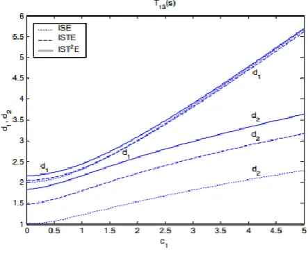
_dfrom (36)

[image:6.595.322.544.455.638.2]

Remarks:

An experienced engineer can use the above given guidelines to determine the four tuning parameters of the PI-PD controller and also there are four tuning parameters of the PI-PD controller, it requires more effort to obtain suitable tuning parameters

Fig. 3. Optimum values of

d

₁and

d

₂for varying

1

c

values

6.

Results

© 2017, IRJET | Impact Factor value: 5.181 | ISO 9001:2008 Certified Journal | Page 263

Example 1

Consider a first order time delay system;

1

₅

(

s



1)

. The

model used for the designing PI controller is

2.93

1 2.73

s

e

s





.

Now the proposed tuning method gives the following PI/PID controllers parameters

(





0.7)

.

:

0.6196,

0.1983

:

0.9665,

0.2704,

0.8463

p i

p i d

PI k

k

PID k

k

k











For comparison, results are presented for the PI controller by Ziegler-Nichols method [8,9] control parameters are

:

p

0.83856,

i

0.1023

Z



N k



k



. And also Gain and Phase

Margin method, control parameters are

(

A

_m



3,



_m



60)

.GPMPI k: p0.4878,ki0.1787

Simulation results:

0 10 20 30 40 50 60 70 80 90 100

0 0.2 0.4 0.6 0.8 1 1.2 1.4 1.6 1.8

Time

A

m

p

li

tu

d

e

NA-PI NA-PID GPM-PI Z-N

0 10 20 30 40 50 60 70 80 90 100

-0.1 0 0.1 0.2 0.3 0.4 0.5 0.6 0.7 0.8

Time

A

m

p

li

tu

d

e

[image:7.595.307.547.335.527.2]

NA-PI NA-PID GPM-PI Z-N

Fig. 4. Unit step response and load-disturbance response of Numerical PI, Numerical PID, GPM-PI, and

Ziegler-Nichols controller.

Comparison results shown in Fig. 4. For unit step response and load-disturbance response, respectively. It observed that the performance of Numerical PI/PID controller method is better than that of Z-N method, and GPM-PI method

6.1. Kharitonov Rectangular theorem for robust

analysis

We know that for the robustness analysis of control systems with parametric uncertainty kharitonov theorem and related approaches can be used

Let us consider Example 2 of this paper. Here two cases will be considered in order to compare how the robustness of the closed-loop system is affected by the choice of PI controller gain K_p. From (32) the closed loop

characteristic equation of proposed control structure.



1 2



( ) 1

s

G s K s

_m

( )

( )

K s

( )

0



 





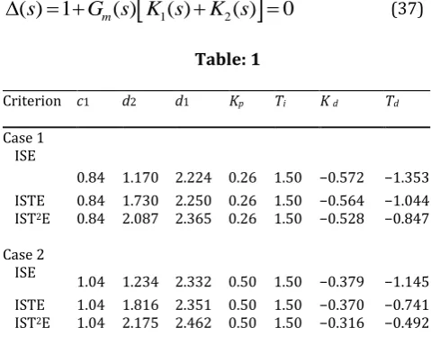
(37)

Table: 1

Criterion c1 d2 d1 Kp Ti K d Td

Case 1 ISE

0.84 1.170 2.224 0.26 1.50 −0.572 −1.353 ISTE

IST2E

0.84

0.84 1.730 2.087 2.250 2.365 0.26 0.26 1.50 1.50 −0.564 −0.528 −1.044 −0.847 Case 2

ISE _{1.04 1.234 2.332 0.50 1.50 −0.379 −1.145} ISTE

IST2E

1.04

1.04 1.816 2.175 2.351 2.462 0.50 0.50 1.50 1.50 −0.370 −0.316 −0.741 −0.492

Initially consider case 1. From Table 1, note that the controllers correspond to the 2

IST E

criterion. we can

write

K s

₁

( )



0.26(1 1 1.5 )



s

and

K s

₂

( )

 

0.528 0.847



s

Substitute these in (37). Now the closed loop characteristic equation is given as

3 2

( )s 1.5s (1.5a 1.27 )k s (1.5b 0.402 )k s 0.26k

       =0

(38)

Nominal values of system transfer function from example 2. k=1, a=2, b=1. It is assumed that

k



[0.9,1.1],

a



[1.6, 2.4]

and b[0.7,1.3]. Therefore, the following interval

characteristic polynomial can be obtained as

3 2

( )s 1.5s (1, 2.457)s (0.61,1.59)s (0.234, 0.249) 0

     

© 2017, IRJET | Impact Factor value: 5.181 | ISO 9001:2008 Certified Journal | Page 264

Now the four Kharitonov polynomial are found to be

2 3

1

2 3

2

2 3

3

2 3

4

( )

0.234 0.61

2.457

1.50

( )

0.234 1.59

2.457

1.50

( )

0.249 0.61

1.00

1.50

( )

0.249 1.59

1.00

1.50

K s

s

s

s

K s

s

s

s

K s

s

s

s

K s

s

s

s

































(40)

Similarly, now consider case 2.

Where,

1( ) 0.50(1 1 1.5 )

K s   s ,K s₂( ) 0.316 0.492 s

Substitute these in (37). Now the closed loop characteristic equation is given as,

3 2

( ) 1.5s s (1.5a 0.738 )k s (1.5b 0.7026 )k s 0.50k

      

(41)

And the following interval characteristic polynomial can be obtained as,

3 2

( ) 1.5s s (1.588, 2.936)s (1.30, 2.254)s (0.45, 0.55) 0

     

(42)

Now the four Kharitonov polynomial are found to be

2 3

1

2 3

2

2 3

3

2 3

4

( )

0.45 1.30

2.936

1.50

( )

0.45 2.254

2.936

1.50

( )

0.55 1.30

1.588

1.50

( )

0.55 2.254

1.588

1.50

K s

s

s

s

K s

s

s

s

K s

s

s

s

K s

s

s

s

































(43)

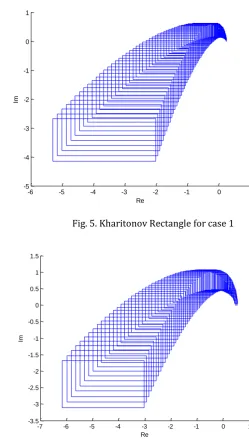
[image:8.595.298.548.103.543.2]

Roots of Kharitonov polynomials for both cases are in negative real parts and hence satisfy Hurwitz condition. And Kharitonov rectangles of the closed loop system are given in Fig.4 and 5for case 1 and case 2, respectively. It can be seen that the Kharitonov rectangles do not include the origin. Therefore, from zero exclusion principle one can say that the interval characteristic equations for both cases are stable. Thus, designed controllers for two cases are robust.

-6 -5 -4 -3 -2 -1 0 1

-5 -4 -3 -2 -1 0 1

Re

Im

Fig. 5. Kharitonov Rectangle for case 1

-7 -6 -5 -4 -3 -2 -1 0 1

-3.5 -3 -2.5 -2 -1.5 -1 -0.5 0 0.5 1 1.5

Re

[image:8.595.311.547.111.310.2]

Im

Fig. 6. Kharitonov Rectangle for case 2

From Fig.5 and 6 it can be seen that the value set for the first case is closer to origin then the second case. Then it is concluded that the controller design for second case is more robust than the first case.

Example 2

Consider a non-minimum phase zero model;

1

₃

(

1)

s

s





. The

model used for the designing PID controller is

1.58 2

(

1)

s

e

s





. Now

[image:8.595.317.550.345.540.2]

© 2017, IRJET | Impact Factor value: 5.181 | ISO 9001:2008 Certified Journal | Page 265

: p 0.7983, i 0.3514, d 0.4497

PID k  k  k  . For comparison,

results are presented for the PID controller by Gain and Phase Margin method, control parameters are

(Am3,



m60)PID k: p0.7983,ki0.3514,kd 0.4497.

And also, PI-PD control parameters are,

: _p 0.50, _i 0.18703, _d 1.6966

PIPD k  k  k 

.

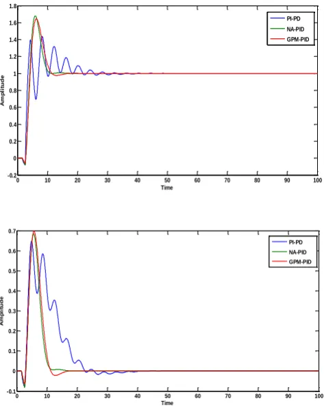
Simulation results:

0 10 20 30 40 50 60 70 80 90 100

-0.2 0 0.2 0.4 0.6 0.8 1 1.2 1.4 1.6 1.8

Time

A

m

p

li

tu

d

e

PI-PD NA-PID GPM-PID

0 10 20 30 40 50 60 70 80 90 100

-0.1 0 0.1 0.2 0.3 0.4 0.5 0.6 0.7

Time

A

m

p

li

tu

d

e

[image:9.595.44.281.231.532.2]

PI-PD NA-PID GPM-PID

Fig. 7. Unit step response and load-disturbance response of Numerical PID, GPM-PID, and PI-PD controller

Comparison results shown in Fig. 7. For unit step response and load-disturbance response, respectively. It observed that the performance of Numerical PID controller method is superior than that of GPM-PID method and PI-PD controller method.

7.

Conclusion

This paper deals with a simple robust PI/PID controller design method developed using numerical optimization approach for time delay systems. And also, different examples and simulation results demonstrated the effectiveness of the proposed approach when compared with GPM, Ziegler-Nichols, and PI-PD controller methods.

8.

References

[1] J. Dawes, L. Ng, R. Dorf, and C. Tam: Design of Deadbeat Robust Systems, Glasgow, UK, 1994, pp. 1597-1598.

[2] D. Valerio, J. Costa: Tuning of Fractional Controllers Minimizing H2 and H∞ Norms, Acta Polytechnica Hungarica, Vol. 3, No. 4, 2006, pp. 55-70

[3] N. Tan: Computation of Stabilizing PI-PD Controllers, International Journal of Control, Automation, and Systems, 7(2), 2009, pp. 175-184.

[4] I.-L. Chien, P.S. Fruehauf, Consider IMC tuning to improve controller performance, Chem. Eng. Progr. (86) (1990) 33–41.

[5] W.K. Ho, C.C. Hang, L.S. Cao, tuning of pid controller based on gain and phase margin specification, Automatica 31 (3) (1995) 497–502

[6] Bhattacharyya SP, Chapellat H, Keel LH (1995) Robust control: the parametric approach. Prentice Hal

[7] Improved Parameter Tuning Methods for Second Order plus Time Delay Processes. K. Venkata Lakshmi Narayana1, Lakshmi Sreekumar2, Sreedevi Edamana3 and Sagari V. S4

[8] The Design of PID Controllers using Ziegler Nichols Tuning Brian R Copeland March 2008.

[9] K.J. Astrom, T. Hagglund, C.C. Hang, W.K. Ho, Automatic € tuning and adaptation for pid controllers-a survey, Contr. Eng. Practice 1 (1993) 699–714

[10]J.J. Di Stefano, A.R. Stubberud, I.J. Williams, Feedback and Control Systems, McGraw-Hill, New York, 1975