Experimental Assessment of the Battery Lifetime in WSN Based on the Duty Cycle Current Average Method

(1)

http://dx.doi.org/10.4236/wsn.2014.610021

Experimental Assessment of the Battery

Lifetime in WSN Based on the

Duty-Cycle

Current Average

Method

Leonardo Barboni1, Maurizio Valle2

1_{Facultad de Ingenieria, Universidad de la Republica, Montevideo, Uruguay}

2_{Department of Naval, Electrical, Electronic and Telecommunications Engineering, University of Genova,}

Genova, Italy

Email: [email protected], [email protected]

Received 25 August 2014; revised 25 September 2014; accepted 24 October 2014

This work is licensed under the Creative Commons Attribution International License (CC BY). http://creativecommons.org/licenses/by/4.0/

Abstract

A great amount of work addressed methods for predicting the battery lifetime in wireless sensor systems. In spite of these efforts, the reported experimental results demonstrate that the du-ty-cycle current average method, which is widely used to this aim, fails in accurately estimating the battery life time of most of the presented wireless sensor system applications. The aim of this pa-per is to expa-perimentally assess the duty-cycle current average method in order to give more effec-tive insight on the effeceffec-tiveness of the method. An electronic metering system, based on a dedi-cated PCB, has been designed and developed to experimentally measure node current consump-tion profiles and charge extracted from the battery in two selected case studies. A battery lifetime measurement (during 30 days) has been carried out. Experimental results have been assessed and compared with estimations given by using the duty-cycle current average method. Based on the measurement results, we show that the assumptions on which the method is based do not hold in real operating cases. The rationality of the duty-cycle current average method needs reconsidering.

Keywords

Battery Lifetime, Current Consumption, TinyOS, Measurement, Duty-Cycle Current Average Method

1. Introduction

(2)

our knowledge, after reviewing the state of the art (by means of well-known bibliographic and citation database of peer-reviewed scientific literature like SCOPUS, EBSCO, JSTOR, IOP science, and IEEE Xplore), we argue that WSN designers avoided carrying out long-term measurements in order to validate battery depletion estimate models for WSN applications. Designers use the duty-cycle current average method, which is nowadays the most accepted method. However, designers often report that batteries are depleted prematurely with respect to the estimation given by such method (e.g. [8]-[12]).

The aim of this paper is to experimentally assess the duty-cycle current average method in order to give more effective insight on the effectiveness of the method. We present a counterexample based on measurements in order to show how the duty-cycle current average method can fail the battery lifetime estimation. As we need a solid understanding of the battery current consumption profile, we have designed an electronic metering system based on a dedicated PCB, which visualizes the node current consumption profile and charge extracted from the battery during the wireless sensor node operation (e.g. transmission, signal sampling). The node used in the ex-periments is the MICAz [13] running applications developed by using nesC language [14]. The TinyOS [15] version is provided by the software platform MOTEWORK [16] and the radio transceiver is the Chipcon CC2420 [17]. The node is powered by two non-rechargeable alkaline IEC-LR6 cells, size AA.

By using the proposed electronic metering system, measurements of two case studies have been performed; the experimental results provide evidence to explain why the duty-cycle current average method is not reliable for the estimation of the battery lifetime. An experimental battery full-depletion time measurement has been conducted to compare the result against the estimation given by the duty-cycle current average method.

2. Wireless Sensor Task and Duty-Cycle Definition

The TinyOs operating system manages the node hardware resources; it is based on the hardware abstraction lay-ers software model (TEP 2 [15]), where each level gives services to upper layers through interfaces. The bottom layer is named Hardware Presentation Layer (HPL) and it is responsible for accessing hardware resources. This is explained in the documented TinyOS Enhancement Proposals also named TEPs (in this case see TEP 2 from [15]). By using this software model, designers can develop programs by using customized interfaces through which the lower hardware abstraction layers are invisible. The WSN application is implemented at the top level (Hardware Interface Layer or HIL). In this framework, the tasks represent applications performed by the wire-less sensor node: e.g. sensor signal sampling, radio transmission and signal processing. The node wakes up (from power down state) in order to execute the task and afterwards goes into sleep mode (power down). In oth-er words, a task is the activity that the node poth-erforms between two powoth-er down states. Each task is executed at the rate R (number of tasks per second) and the task time duration is defined as the active period TA (each task has its own TA). The node duty-cycle time interval D is defined as D=RTA. During the execution of a

task, the node circuit consumes the battery charge

( )

0 d

A

T c

Q =

∫

i t t which is named task charge cost hence-

forth. Figure 1 shows the current consumption profile for a transmission task, where the marked time inter- vals are: interval A

( )

T1 node wake up; interval B

( )

T2 , radio transceiver start-up; interval C

( )

T3 , MAC

layer functions such as channel assessment and backoff-time calculations and receiver system calibration; inter-val D

( )

T5 ,transmission; interval E

( )

T7 ,reception mode according to the MAC protocol [17], waiting for

ACK packets. At the end, the node gets power down state (P.D.), waiting for the next timer interruption for next task execution.

3. Battery Lifetime Estimation Approach

(3)

[image:3.595.191.410.90.204.2]

Figure 1. Battery current profile at −25 dBm output power. Time values are: T₁=0.84 ms,

2 0.58 ms

T = , T₃=2.00 ms, T₄=0.49 ms, T₅=1.1 ms, T₆=0.36 ms, T₇=1.07 ms. The sum is the activity time (or task time) T_A= +T₁ T₂+ +T₃ T₄+ +T₅ T₆+T₇=6.44 ms.

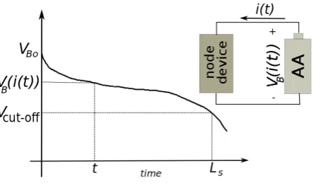
Figure 2. Battery voltage profile; V i t_B

( )

is the battery voltage at time t; V_Bo is the initial

battery voltage, L_S is the node lifetime (service hours) and i t

( )

is the battery current.

tage VB drops below the cut-off voltage Vcutt-off . To estimate the LS value, the node current consumption profile i t

( )

and the equation that relates i t

( )

to the battery voltage, i.e. the equation VB

( )

i t

( )

are needed. The current consumption i t

( )

is determined by the hardware platform and the operating system features.

There has been a lot of effort for building models capable of predicting the current consumption profile i t

( )

, see for instance [18]-[21], but the problem is difficult and not easily tractable.

On the other hand, see for instance [22]-[25], there is no consensus about the description of the battery vol-tage VB

( )

t as function of i t

( )

. Approaches have converged toward the duty-cycle current average method, which is the most widely used to estimate the LS value. The method approximates the node current consump-tion with step-shaped waveforms (named i t s

( )

from herein) that best approximate i t

( )

. The node duty-cycle is assumed to be deterministic and known beforehand. The i ts

( )

integration over the time TA estimates the node charge consumption value. This charge value is then used to estimate the average constant current con-sumption id for such duty-cycle; it is used to estimate the lifetime Ts value by means of the graph constant current discharge vs. hours service, as Figure 3 shows, which is provided by the battery datasheet. From the battery service hours graph it is possible to derive the log-linear relation between the constant current id and the service hours Ts for a given cutoff voltage (e.g. the marked ones with 0.8 V, 1 V and 1.2 V in Figure 3). For example, for the cutoff voltage value 1.2 V, the straight line linking the points (20 mA, 100 h) and (80 mA, 20 h) is as follows:

( )

(

( )

)

10 10 10 10

log T_s −log 20 =m log i_d −log 80 (1)

The coefficient m is given by:

( )

10 10

log 100 log 20 1.2 log 20 log 80

m= − = −

[image:3.595.189.416.263.393.2]

(4)

[image:4.595.177.419.86.227.2]

Figure 3. Battery service hours for different constant current

con-sumption values (figure from [29]).

Then:

( )

10 10 10 10

log Ts =mlog id −mlog 80 +log 20 (3)

( )

10 10

log Ts = −1.2log id +3.51 (4)

Some node platforms vendors provide electronic sheets based on this method; see for example the Mote Bat-tery Life Calculator from Crossbow Technology[26] and other examples given by [27][28]. For examples, in Equation (4) if: 1) id =2.04 mA and 2) id =3.02 mA then respectively: a) Ts =1375.4 h (i.e. 57.3 days)

and b) Ts =859.0 h (i.e. 35.8 days).

To summarize, the hypotheses for using the duty-cycle current average method are the following:

• H1) the node current consumption profile as function of the given application is known. It is a deterministic

waveform that can be always approximated by a step-shaped waveform. The node duty-cycle will be constant during the node lifetime.

• H2) superposition principle: let’s assume that a node performs task 1 with charge cost Qc1 during lifetime

1

s

L . On another hand, let’s assume that the same node performs task 2 with charge cost Qc2 during lifetime

2

s

L . If task 3 is defined as the task 1 plus task 2 (e.g. task 1 performs transmission and task 2 performs signal sampling and data storage, then, task 3 implements both activities, signal sampling, data storage and transmission), the superposition principle states that Qc3 =Qc1+Qc2.

We aim to demonstrate that H1) and H2) hypotheses do not always hold. In the next section, we present the

metering system that has been used to experimentally assess the two hypotheses.

4. Electronic Metering System

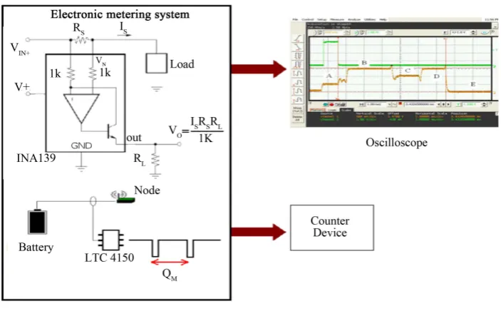
The metering system is based on a dedicated PCB: it visualizes the node current consumption and the task’s charge cost Qc. The prototype PCB is based on the following devices: the High Side Current Shunt Monitor INA139 [30] and the Coulomb Counter LTC4150 [31]. Figure 4 shows the metering system block diagram. The INA139 amplifies the voltage across a shunt resistance between battery and load. The measured voltage is pro-portional to the battery current consumption. The output voltage signal is in input to an amplification stage and subsequently to an oscilloscope where the current waveform associated to the node task can be analyzed. The shunt resistance value has been selected so that the INA139 gain provides the maximum output voltage range at the maximum node current consumption. The board is powered by a 3 V voltage. The charge counter characteriz-es the node in terms of consumed charge; valucharacteriz-es are exprcharacteriz-essed in charge units (mAh or μAh). The LTC4150 de-vice is a voltage integrator with a voltage-to-frequency converter. The coulomb counter dede-vice forces to zero the output pin voltage when a fixed quantity of charge QM has been measured.

(5)

[image:5.595.123.475.82.300.2]

Figure 4. Block diagram of the experimental setup.

executes N times the same task during the time T, we estimate the average task charge cost value Qc as Equation (5), where N is such that N= ⋅R T (the measurement ends when time T is reached and the task has been executed N times).

T M

c

Q KQ Q

N N

= = (5)

The error is given by Equation (6) where ∆ =K 1

M c

K Q Q

N ∆ ⋅

∆ = (6)

We use the following example to illustrate the methodology. If the node performs packet transmissions at the rate R=10 packets/s, for a given time, e.g. T = 3600 s, the number of performed tasks (equal to the number of packet transmissions) is N=36000. If we count, for instance, K =1000 pulses, from Equation (5) the charge cost associated to the transmission task and the related error result as follows:

5.2 μAh

1000 144.4 uAh 36000

c

Q = × = (7)

5.2 μAh

144.4 pAh 0.15 nAh 36000

c Q

∆ = =  (8)

As a final remark, we observe that the best set of values

{ }

T R, to perform the experiment is such that 1

N values (e.g. 1000 or more), in order to meet the condition ∆Qc Qc. The proposed method has the disadvantage that it requires long time measurements. A suitable value of T (or N) is not known a priori, because the value Qc is obviously not known, as well as the K value. This problem can be overcome with an iterative procedure, by performing several measurements. In general from our experience, we have not conducted mea-surement of more than 4 hours. In this article, the node tasks under evaluation are transmissions (task 1) and temperature sensor sampling (task 2). The measured amount of charge Qc for each task is shown in Table 1.

5. Battery Lifetime Time Measurement

The MICAz node has been programmed to transmit one packet with a payload of 25 bytes, at the output power level of −25 dB∙m. The transmission rate is 1

20 s

(6)

below 2.4 V (i.e. individual cell voltage value of 1.2 V). We daily measured the battery voltage and the result is shown in Figure 5; the voltage value 2.4 V has been achieved in 30 days.

The current consumption profile has been measured during transmission; it is shown in Figure 1. The result-ing duty-cycle is D=6.44 ms 50 ms=0.13. In accordance with the duty-cycle current average method, it is assumed that this current profile is repeated each time that the radio performs a transmission. By numerical inte-gration, the average discharge current inside the duty-cycle time interval is given by i_d =2.04 mA; the esti-mated battery lifetime (Equation (4)) is Ts =1375.4 hs, i.e. 57.3 days, with an error of27 days with respect to the measured one. At this point, it is necessary to understand why there is such big difference between estimated and measured results. To this aim, we used the metering system for visualizing the node current consumption profile.

6. Assessment of

H

1

Hypothesis

Differently to the previously presented lifetime estimate, we use Qc = 0.042 μAh (see Table 1). The average current consumption is id =Qc 50 ms=3.02 mA and by means of Equation (4), the estimated lifetime is

859.0 h s

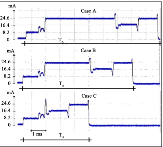
T = (i.e. 35.8 days), which is a better approximation with respect to the previous one. We conclude that the H1 hypothesis does not hold. The metering system provides excellent accuracy to measure Qc for large N values. It is not necessary to assume any node current consumption profile beforehand and the overall current consumption is taken into account to measure Qc (including node start-up and power down states). The reduced current consumption levels are frequently neglected in the duty-cycle current average method, never-theless, they could have cumulative effects during the node lifetime. It is not enough to observe the current con-sumption profile for a short time to estimate the real required charge Qc because our measurements shows non periodic current consumption profile. In fact, we observed a time-varying duty cycle (time-varying current con-sumption). Figure 6 shows three different observed cases, among others. The difference between duty-cycle values of cases A and C is 48.9%. Then, it is not possible to have a deterministic known current profile during transmissions and the H1 hypothesis which states that the duty-cycle is constant, does not hold.

Therefore, without a reliable value of the duty cycle value, the duty-cycle current average method can esti-mate the lifetime value very roughly. In fact, it is not possible to assume a priori node current consumption pro-file and the experimental characterization should be done for every given application. The node tasks are con-trolled by the program that runs inside the microcontroller under the supervision of an operating system like TinyOS [14]. Most of the time, the operating system asynchronously manages hardware resources in order to provide services to asynchronous events related to the wireless communication. More specifically, the origin of this non deterministic behavior is given by the method used for the clear channel assessment in most of the MAC layer protocols (see Chapter 5 MAC Protocols in [20]). Therefore, generally speaking, the node awakes and sleeps in a non-deterministic way and the battery is forced to deliver current patterns which are not easily predictable, neither the duty-cycle value. The duty-cycle current average method requires the knowledge of the deterministic node current consumption, but we assessed that it is not possible.

7. Assessment of

H

2

Hypothesis

Table 1 shows charge costs for the tasks 1 and 2. Task 3 is defined as the sampling plus the transmission tasks, i.e. the node performs signal sampling and then packet transmission. The H2 hypothesis states that the expected

battery charge cost Qc3 for task 3 should be equal to the sum of Qc1 (task 1) and Qc2 (task 2). To verify the

H2 hypothesis, we implemented the task 3 and experimental measurements have been performed.

(7)

[image:7.595.107.488.82.270.2]

Figure 5. Measured battery voltage during node transmissions.

Figure 6. Three different measurements that show the time-varying node current profile behavior because of the random nature of backoff-time calculation for the MAC layer. Please, note how the TA value varies.

Case A: D≈9.2 ms 50 ms or 18.4%; Case B: D≈7.5 ms 50 ms or 15.0%; Case C: D≈4.5 ms 50 ms

[image:7.595.154.487.158.525.2]

or 9.0%.

Table 2. Measured charge Qc.

Task Charge cost Qc[μAh]

Task 1 + Task 2 0.520 + 0.042 = 0.560

Task 3 2.04

nificantly different with respect to the expected ones.

[image:7.595.167.431.294.532.2]

(8)

electronic metering system, based on a dedicated PCB to experimentally measure node current consumption profiles and charge extracted from the battery for two selected case studies, has been designed and implemented. Based on the measurement results, we demonstrate that the hypotheses on which the method is based are not re-liable. The concluding remarks to be taken into account for the development of WSN applications are: 1) the software architecture and how to develop the application program have strong influence on the node current consumption profile and hence, on the battery lifetime; 2) the node current consumption profile as function of the given application as well as the duty-cycle is not deterministic. The duty-cycle current average method has another hypothesis which has not been considered: the battery operating temperature, which would have signifi-cant effect on the graph constant current discharge vs. hours service. It should be addressed as future research trend.

References

[1] Lu, B. and Gungor, V.C. (2009) Online and Remote Motor Energy Monitoring and Fault Diagnostics Using Wireless Sensor Networks.IEEE Transactions on Industrial Electronics, 56, 4651-4659.

http://dx.doi.org/10.1109/TIE.2009.2028349

[2] Gungor, V.C. and Gerhard, P.H. (2009) Industrial Wireless Sensor Networks: Challenges, Design Principles, and Technical Approaches. IEEE Transactions on Industrial Electronics, 56, 4258-4265.

[3] Dondi, D., et al. (2008) Modeling and Optimization of a Solar Energy Harvester System for Self-Powered Wireless Sensor Networks. IEEE Transactions on Industrial Electronics, 55, 2759-2766.

[4] Agha, K.A., et al. (2009) Which Wireless Technology for Industrial Wireless Sensor Networks? The Development of OCARI Technology. IEEE Transactions on Industrial Electronics, 56, 4266-4278.

[5] Ahn, H.-S. and Ko, K.H. (2009) Simple Pedestrian Localization Algorithms Based on Distributed Wireless Sensor Networks. IEEE Transactions on Industrial Electronics, 56, 4296. http://dx.doi.org/10.1109/TIE.2009.2017097

[6] Pierce, F.J. and Elliott, T.V. (2008) Regional and On-Farm Wireless Sensor Networks for Agricultural Systems in Eastern Washington. Computers and Electronics in Agriculture, 61, 32-43.

http://dx.doi.org/10.1016/j.compag.2007.05.007

[7] Lopez, J.A., et al. (2009) Development of a Sensor Node for Precision Horticulture. Sensors, 9, 3240-3255.

http://dx.doi.org/10.3390/s90503240

[8] Torvmark, K.H. Low Power Systems Using the CC1010. Chipcon Application Note AN017.

[9] Baleri, G. Guidelines for WSN Design and Deployment.

http://www.aolsearch.com/search?s_it=searchbox.webhome&s_gl=CN&v_t=na&q=%5B9%5D%09GiriBaleri%2C+Cr ossbow+Technology%2C+Inc.+Guidelines+for+WSN+Design+and+Deployment

[10] The Battery Life Estimator. A Web-Based Calculator to Help Optimize Low-Power Applications.

http://www.silabs.com/support/pages/batterylifeestimator.aspx

[11] Yang, O. and Heinzelman, W.B. (2012) Modeling and Performance Analysis for Duty-Cycled MAC Protocols with Applications to S-MAC and X-MAC. IEEE Transactions on Mobile Computing, 11, 905-921.

http://dx.doi.org/10.1109/TMC.2011.121

[12] Jiang, X.,Taneja, J., Ortiz, J., Tavakoli, A., Dutta, P., Jeong, J., et al. (2007) An Architecture for Energy Management in Wireless Sensor Networks. Special Issue on the Workshop on Wireless Sensor Network Architecture, 4, 31-36.

(9)

[14] Gay, P., Welsh, M., Levis, P., Brewer, E., Von Behren, R. and Culler, D. (2003) The nesC Language: A Holistic Ap-proach to Networked Embedded Systems. Proceedings of the ACM SIGPLAN 2003 Conference on Programming Language Design and Implementation, San Diego, 9-11June 2003.

[15] http://tinyos.stanford.edu/tinyos-wiki/index.php/TinyOS_Documentation_Wiki

[16] MoteWork Crossbow—Platform for the Development of Wireless Sensor Network from Crossbow.

www.willow.co.uk/MoteWorks_OEM_Edition.pdf

[17] CC2420 2.4 GHz IEEE 802.15.4 ZigBee-Ready RF Transceiver Chipcon, Product from Texas Instruments.

http://focus.ti.com/docs/prod/folders/print/cc2420.html

[18] Kan, B., Cai, L., Zhao, L. and Xu, Y. (2007) Energy Efficient Design of WSN Based on an Accurate Power Consump-tion Model. Proceedings of theWireless Communications, Networking and Mobile Computing (WiCom 2007), Shang-hai, 21-25 September 2007, 2751-2754.

[19] Barberis, A., Barboni, L. and Valle, M. (2007) Evaluating Energy Consumption in Wireless Sensor Networks Applica-tions. Proceedings of the 10th Euromicro Conference on Digital System Design Architectures, Methods and Tools, Lu- beck, 29-31 August 2007, 455-462. http://dx.doi.org/10.1109/DSD.2007.4341509

[20] Holger, K. and Willig, A. (2005) Protocols and Architectures for Wireless Sensor Networks. John Wiley & Sons, Ho-boken.

[21] Bougard, B., Daly, D.C., Chandrakasan, A. and Dehaene, W. (2005) Energy Efficiency of the IEEE 802.15.4 Standard in Dense Wireless Microsensor Networks: Modeling and Improvement Perspectives. Proceedings of the Conference on Design, Automation and Test, 1, 196-201.

[22] Rao, R., Vrudhula, S. and Rakhmatov, D. (2003) Battery Modeling for Energy-Aware System Design. IEEE Computer Society, 36, 77-87. http://dx.doi.org/10.1145/860176.860179

[23] Rakhmatov, D. and Vrudhula, S. (2003) Energy Management for Battery-Powered Embedded Systems. ACM Transac-tions on Embedded Computing Systems, 2, 277-324. http://dx.doi.org/10.1145/860176.860179

[24] Rao, R., Vrudhula, S. and Chang, N. (2005) Battery Optimization vs Energy Optimization: Which to Choose and When?

Proceedings of Conference on Computer-Aided Design, ICCAD IEEE/ACM,San Jose, 6-10 November 2005, 439-445.

[25] Panigrahi, D., Chiasserini, C., Dey, S., Rao, R., Raghunathan, A. and Lahiri, K. (2001) Battery Life Estimation of Mo-bile Embedded Systems. Proceedings of 14th International Conference on VLSI Design (VLSID 01),Bangalore, 3-7 January 2001, 57-63.

[26] Expected Battery Life vs. System Current Usage and Duty Cycle, PowerManagement.xls. Excel Worksheet from Crossbow Technology. http://www-db.ics.uci.edu/pages/research/quasar/PowerManagement.xls

[27] Kyaw, Z.T. and Sen, C. (2008) Using the CC2430 and TIMAC for Low-Power Wireless Sensor Applications: A Power Consumption Study. http://focus.ti.com.cn/cn/lit/an/slyt295/slyt295.pdf

[28] Application Note AN053 Measuring Power Consumption with CC2430 and Z-Stack.

http://focus.ti.com/lit/an/swra144/swra144.pdf

[29] Product Datasheet Energizer E91, Alkaline Battery AA. Energizer Holdings, Inc. Form No. EBC-1202M.

http://www.energizer.com/

[30] High-Side Measurement Current Shut Monitor INA 139, Datasheet Burr-Brown Products from Texas Instruments.

http://focus.ti.com/

(10)