Image Compression using DPCM with LMS Algorithm

(1)

© 2017, IRJET | Impact Factor value: 5.181 | ISO 9001:2008 Certified Journal

| Page 824

Image Compression using DPCM with LMS Algorithm

Reenu Sharma, Abhay Khedkar

SRCEM, Banmore

---****---

Abstract: The Differential pulse code modulation (DPCM) [1] may be used to remove the unused bit in the image for image compression. In this paper we compare the compressed image for 1, 2, 3, bit and also compare the estimation error. The LMS [2] Algorithm may be used to adapt the coefficients of an adaptive prediction filter for image source coding. In the method used in this paper we decrease the compressed image distortion and also the estimation error. The estimation error is reduced as much as 7-8 dB using DPCM with LMS Algorithm.

Key Words: - Adaptive filter, LMS algorithm, DPCM, Quantization.

1. INTRODUCTION

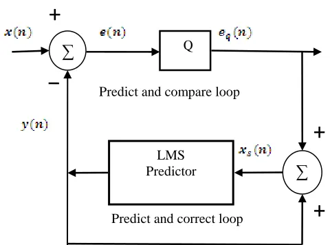
In a communication environment, the difference between adjacent time samples for image is small, coding techniques have envolved based on transmitting sample-to-sample differences rather than actual sample value. Successive differences are in fact a special case of a class of non-instantaneous converters called N-tap linear predictive coders. These coders, sometimes called predictor-corrector coders, predict the next input sample value based on the previous input sample values. This structure is shown in figure 1. In this type of converter, the encoder forms the prediction error (or the residue) as the difference between the next measured sample value and the predicted sample value. The equation for the prediction error [3] is

1.1 In figure 1: Where Q=Quantizer, is the nth input sample, is the predicted value, and is the associated prediction error. This is performed in the predict-and-compare loop, the loop shown in figure 1. It’s prediction by forming the sum of its prediction and the prediction error

1.2

Where quant (.) represents the quantization operation, is the quantization [4] version of the prediction error, and is the corrected and quantized version of the input sample. This is performed in the predict-and-correct loop.

∑

Q

LMS

Predictor

∑

+

Predict and compare loop

[image:1.612.316.556.495.673.2]

Predict and correct loop

+

(2)

[image:2.612.76.234.108.273.2]

© 2017, IRJET | Impact Factor value: 5.181 | ISO 9001:2008 Certified Journal

| Page 825

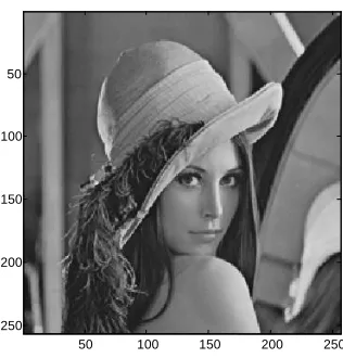
Figure 2 Original image

The communication task is that of transmitting the difference (the error signal) between the prediction and the actual data sample. For this reason, this class of coder is often called a differential pulse code modulator (DPCM) [3]. If the prediction model forms predictions that are close to the actual sample values, the residues variance (relative to the original signal).

2. ANALYSIS OF DPCM

In DPCM [3] we transmit not the present sample x(n), but e(n) (the difference between x(n) and its predicted value y(n)). At the receiver, we generate y(n) from the past sample value to which the received x(n) is added to generate x(n). There is, however, one difficulty associated with this scheme. At the receiver, instead of

the past samples as well as we

have their quantized version this will increase the error in reconstruction. In such a case, a better strategy is to determine the estimate of (instead of ), at the transmitter also from the

quantized samples difference e(n)=x(n)-y(n) is now transmitted via PCM. At the receiver, we can generate and from the received we can reconstruct Figure 1 shown a DPCM predictor. We shall soon show that the predictor input is Naturally, its output is the predicted value of The difference of original image data, and prediction image data, is called estimation residual, . So

2.1 is quantized to yield

Where is the quantization error, quantized signal. And

2.2 The prediction output is fed back to its input so that the predictor input is

2.3 This shows is quantized version of The prediction input is indeed , as assumed. The quantized signal is now transmitted over the channel.

3. IMAGE COMPRESSION USING DPCM AND

LMS ALGORITHM

A block diagram of the LMS adaptive image compression system is shown in figure 1. It is seen that the image prediction is formed in a linear manner at the output of the LMS filter:

50 100 150 200 250

50

100

150

200

(3)

© 2017, IRJET | Impact Factor value: 5.181 | ISO 9001:2008 Certified Journal

| Page 826

3.1

3.2

In equation 3.2, the are N adaptive predictor coefficients, the are the reconstructed image data, and k is 1, 2……….N integer values which select the previous image pixel on which base the current prediction. At each scanned pixel a prediction residual (error), is computed

3.4

This quantized residual is send to the receiver. The quantization residual is determine

3.5

This residual is then quantized to form and the quantized residual is also used to update the predictor coefficient for the next iteration by the well known least mean squares (LMS) [5] algorithm.

3.6

The parameter µ is known as the step size parameter and is a small positive constant, which control steady-state and convergent mean-square residual characteristics of the predictor. The LMS algorithm is an approximation to the gradient search method for iteratively computing the N optimal coefficients which minimize the mean square prediction residual. It is known by [6] that the error between the original image and the reconstructed image at the receiver is simply the quantization error Thus, the distortion

between the original discrete image x(n) and the

reconstructed value y(n) at the receiver is given by

3.7

(Assuming the no channel-induced errors)

Therefore, if the goal of the system is an accurate reconstruction of the image, then an algorithm is desired which will form an accurate so that e(n) will have smaller variance and the quantizer levels may be adjusted to give a smaller quantization error.

Hence, a lower reconstruction error, or distortion, will be present at the receiver. The quantizer levels themselves may be fixed or may vary as some function of the residual sequence . Although, in general, the position of the quantizer levels could be adaptive, for simplicity, in this correspondence we only examine the case of a quantizer with fixed levels.

Alternatively, if the goal of the system is to reduce the bit rate over the channel subject to some distortion criteria, then we may reduce the number of quantizer levels which span the residual signal range and, hence, produce shorter code words per level. In this situation the LMS adaptive predictor reduces the average number of bits per image while maintaining an acceptable visual appearance at the receiver.

4. SIMULATION RESULT

(4)

© 2017, IRJET | Impact Factor value: 5.181 | ISO 9001:2008 Certified Journal

| Page 827

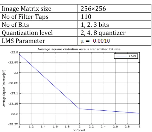
DPCM image quantization [8], [9]. The dynamic range of

data was eight bits from grey level 0 to 255. The figure 3 plots the average square distortion versus transmitted bit rate for the woman image. All values of average square error are in dB referenced to the performance of the 1bits/pixel fixed coefficient predictor. The bit rate is in bits/pixel and is controlled by the number of levels in the quantizer. If number of bit increasing and distortion will be decrease. Figure 7, 8, and 9 is shown the prediction mean square versus gray level respectively for 1, 2, and 3 bits reconstructed image. And figure 10 is shown the comparison of PMSE. If the number of bits is increasing then PMSE will be decreasing.

Table 1 Condition in Simulation Experiment

Image Matrix size 256×256 No of Filter Taps 110

No of Bits 1, 2, 3 bits

Quantization level 2, 4, 8 quantizer

LMS Parameter

1 1.2 1.4 1.6 1.8 2 2.2 2.4 2.6 2.8 3

-23.25 -23.2 -23.15 -23.1 -23.05 -23 -22.95 -22.9

Average square distortion versus transmitted bit rate

A

ve

ra

ge

S

qu

ar

e

D

is

to

rt

io

n[

dB

]

bit/pixel

[image:4.612.43.297.388.608.2]

LMS

Figure 3 average square distortions versus transmitted bit rate.

50 100 150 200 250

50

100

150

200

250

50 100 150 200 250

50

100

150

200

250

50 100 150 200 250

50

100

150

200

250

Figure 4 1bits/pixel LMS images

[image:4.612.359.530.518.677.2]

Figure 5 2bits/pixel LMS images

(5)

| Page 828

0 50 100 150 200 250 300

-46 -44 -42 -40 -38 -36 -34 -32 -30 -28 -26

PMSE of LMS Algorithm

P M S E [ dB ] sample number 1bit

Figure 7 PMSE [dB] versus Sample number for 1bits/sample

0 50 100 150 200 250 300 -65 -60 -55 -50 -45 -40 -35 -30

P M S E [d B ] sample number 2bit

Figure 8 PMSE [dB] versus Sample number for 2bits/sample.

0 50 100 150 200 250 300 -75 -70 -65 -60 -55 -50 -45 -40 -35 -30

[image:5.612.321.554.102.231.2]

P M S E [d B ] sample number 3bit

Figure 9 PMSE [dB] versus Sample number for 3bits/sample.

0 50 100 150 200 250 300 -75 -70 -65 -60 -55 -50 -45 -40 -35 -30 -25

Comparision of PMSE For 1,2,3 Bits

[image:5.612.47.280.105.261.2]

P M S E [d B ] sample number 1bit 2bit 3bit

Figure 10 PMSE [dB] versus Sample number for 1, 2, 3 bits/sample comparison.

5. CONCLUSSION

The LMS is a simple and robust adaptive algorithm and DPCM use the LMS for prediction. At last the distortion is reduce for 1, 2, 3 bits and also reduce the estimation mean square error. The distortion and the estimation mean square error is very less. We compare the estimation mean square error in dB. This difference is 7-9 dB respectively for 1, 2, 3 bits as shown in figure 10 and the reduce image shown in figure 4, 5, and 6 respectively this work carried out in future also.

REFERENCES

[1]. A. Habbi, “Comparison of Nth-order DPCM encoder with linear transformation and block quantization techniques,” IEEE Trans. Commun., vol. COM-19, pp. 948-956, Dec. 1971.

[2]. S.Haykin and T.Kailath “Adaptive Filter Theory” Fourth Edition. Prentice Hall, Pearson Eduaction 2002.

[3]. B. P. Lathi and Zhi ding “Modern Digital and Analog Communication Systems” International Fourth Edition. New York Oxford University Press-2010, pp.292.

[4]. J. E. Modestino, and D. G. Daut, “Source-channel coding of images,” IEEE Trans. Commun., vol. COM-27, pp. 1644-1659, Nov. 1979.

[image:5.612.50.278.318.447.2] [image:5.612.48.278.501.641.2]

(6)

| Page 829

Acoust., Speech, Signal Processing, vol. ASSP-26, pp.

240-254, June 1978.

[6]. J. G. Prokis, Digital Communications. New York: McGraw-Hill, 1983.

[7]. S. T. Alexander and S. A. Rajala, “Analysis and simulation of an adaptive image coding system using the LMS algorithm,” in Proc. 1982 IEEE Int. Conf. Acoust., Speech Signal Processing, Paris, France, May 1982.

[8]. W. K. Pratt, Digital Image Processing. New York: Wiley, 1978.

[9]. J. E. Modestino, and D. G. Daut, “Source-channel coding of image,” IEEE Trans. Commun., vol. COM-27, pp. 1644-1659, Nov1979.