http://dx.doi.org/10.4236/wjet.2015.33C044
Valuation of Asian American Option Using a
Modified Path Simulation Method
Ferry Jaya Permana, Dharma Lesmono, Erwinna Chendra
Department of Mathematics, Universitas Katolik Parahyangan, Bandung, Indonesia Email: [email protected], [email protected], [email protected]
Received 12 September 2015; accepted 15 October 2015; published 22 October 2015
Abstract
In this paper, we use a modified path simulation method for valuation of Asian American Options. This method is a modification of the path simulation model proposed by Tiley. We assume that the behavior of the log return of the underlying assets follows the Variance Gamma (VG) process, since its distribution is heavy tail and leptokurtic. We provide sensitivity analysis of this method and compare the obtained prices to Asian European option prices.
Keywords
Asian American Option, European American Option, Variance Gamma Process, Path Simulation Model
1. Introduction
In the recent years, option has become one of well-known financial instruments for hedging strategy. In the fi-nancial market, hundreds of options are traded daily. For some cases, options are specifically customized to hedge the market risk of underlying assets and to response market players’ demand. The customized options are developed based on the characteristics of underlying assets. For example, the famous Black-Scholes model is re-lied on assumption that the underlying asset price dynamic follows the Geometric Brownian motion (GBM). It means that the log return of asset is normally distributed. This model is widely used to determine the price of European and American options.
challeng-ing task.
The contribution of this paper is to determine the price of Asian option using VG model and compare option prices between an Asian European and Asian American option according to some performance criteria. We also develop a new approach by using the conditional distribution of the VG process to determine the price of Asian European options. To price Asian American options, we apply the modified path simulation method based on Tiley [4] which is similar to valuation of American options. In deriving the method, Tiley [4] assumed that the underlying asset price dynamics follow the GBM. Performance of the modified path simulation method applied to Asian American options is investigated by comparing the obtained Asian American option prices to the Asian European option prices. Comparison in terms of option prices is also provided with the plain vanilla European option and plain vanilla American option.
The organization the rest of this paper is as follows. In Section 2, we describe Asian option, while the modi- fied path simulation method for Asian American option is given in Section 3. Simulation study is given in Sec-tion 4 and in the last secSec-tion we give conclusions and further research.
2. Asian Option
Asian option is an option whose payoff depends on the arithmetic average price of underlying asset over a cer-tain period of time, from the initiation of the contract until its maturity date. It is assumed that the underlying asset price dynamics follow the VG process, under the risk-neutral process. By considering the discrete avera- ging times: t0=0, , ,t t1 2 …,tN =T, where T is the time to maturity, the underlying asset price at time ti, de-noted by S t
( )
i , is given as follows( )
i( )
0 exp(
i(
i; , ,)
i)
S t =S rt +X t
σ υ θ
+ω
tThe arithmetic average price of underlying asset at time ti, denoted by A t
( )
i , is defined as:( )
0( )
1 1
i
i j j
A t S t
i =
=
+
∑
where i=0,1, 2,…, .N The payoff of European Asian option with the strike price K is given by:
( )
(
)
payoff of call option=max A T −K, 0
( )
(
)
payoff of put option=max K−A T , 0 .
The existing methods to determine the price of a European option, (see for example Madan and Milne [5]) cannot be directly applied for Asian option. The reason is the arithmetic average of variables following the VG process does not follow the VG process. The easiest way to value the Asian European option is to apply the Monte Carlo simulation. First, we generate a finite sample of R underlying asset paths whereeach path has N epochs. It is assumed that the k-th path in the sample is represented by the sequence:
( ) ( ) ( )
, 0 , ,1 , , 2 , , ( , )S k S k S k … S k N . Namely S k j
( )
, is S t( )j at the k-path. For the k-th path we will have the sequence of the Arithmetic average prive:( ) ( ) ( )
, 0 , ,1 , , 2 , , ( , )A k A k A k … A k N
where
( )
( )
0 1
, ,
1
i j
A k i S k j
i =
=
+
∑
. By using that path, we can value the European Asian call and put options asfollows:
(
)
(
(
)
)
exp max( , , 0)
c= −rT E A k N −K
(
)
(
(
)
)
exp max( , , 0)
c= −rT E A k N −K .
3. Modified Path Simulation Method for Asian American Option
One approach to determine the price of the American option is using simulation. However, many literatures found that simulation such as Monte Carlo simulation, cannot determine the price of the American option effi-ciently (see Dyer and Jacob [6], Geske and Shastri [7], Tiley [8]). Simulation requires large amounts of compu- ter processing time and execution time. Based on this fact, Tiley [4] has developed an algorithm so-called the path simulation model to value the American option more efficiently. In the algorithm, free-arbitrage underlying asset prices are sampled, and the option price is estimated based on these sample paths. In this paper, that ap-proach will be adopted to determine the American option price under the VG process assumption. We call this approach as a modified path simulation method. The procedure for valuing American option using this method can also be found in section 2.3 of [2].
The first step of the algorithm is to generate a finite sample of R underlying asset paths, where each path has N epochs (see Avramidis, L’Ecuyer, P. and Tremblay [9]). It is assumed that the k-th path in the sample is represented by the sequence: S k
( ) ( ) ( )
, 0 ,S k,1 ,S k, 2 ,…, ( ,S k N). For the k-th path we will have the sequence of the arithmetic average price:A k( ) ( ) ( )
, 0 ,A k,1 ,A k, 2 ,…, ( ,A k N), where A k i( ) (
, = 1 /N)
∑
ij=0S k j( )
, . The next step is to reorder the arithmetic asset price paths from the highest to the lowest for an Asian call option or from the lowest to the highest for an Asian put option. We then make partition for the set of R paths into Q distinct bundles of P paths each.Let be defined the intrinsic value I k t( , ) of the option on path k at epoch t
(
t=1, 2,...,N)
as:( )
, max max 0,{
( )
,}
, for call optionfor put option max{0, ( , )},
A k t K
I k t
K A k t
−
=
−
The holding value H k t( , ) is the expectation current value option over all paths in the bundle containing the path-k. Holding values are equal in the same bundles. The core of this algorithm is in determining the path index
*( )
k t as the sharp boundary to decide whether to hold or to exercise the option. The exercise-or-hold variable ( , )
y k t is assume to be 1 for k≥k t*( ), and 0 for k<k t*( ). The indicator variable z k t( , ) is defined as follows
( )
, 1, if( )
, 1 and( )
, 0 for all0, otherwise
y k t y k s s t
z k t = = = <
The current option value equals to intrinsic value when the option is exercised, and equals to holding value when the option is hold. Using backward induction, we can estimate the option price at time 0. However in this algorithm, the accuracy of this estimation depends on partition of the paths we chose.
4. Simulation Study
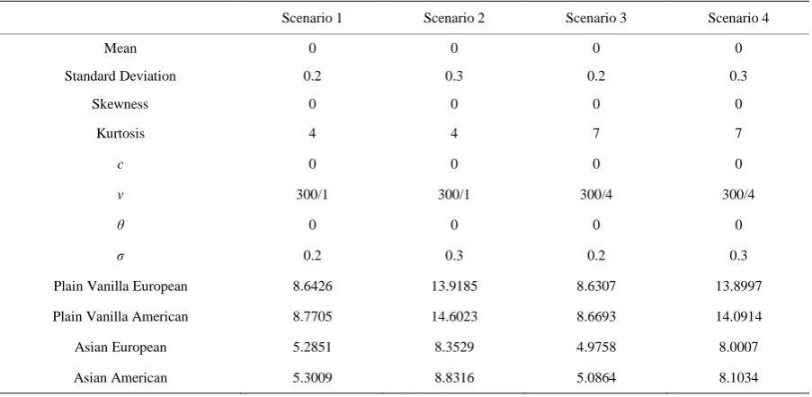
In this section, several scenarios are considered in comparing the option prices for Plain Vanilla European op-tion, Plain Vanilla American opop-tion, Asian European option and Asian American option. Option prices for the Plain Vanilla European option and Asian European option were determined through Monte Carlo simulation, modified path simulation method was employed to determine option prices for the Plain Vanilla American op-tion and Asian American opop-tion. In all of those methods, the parameters we use came from the VG process. In all the scenarios below, we use the value of S(0) = 100 K = 100, T = 1 year and r = 5%/year. The results are given in the table below.
From Table 1, we can conclude that American options always more expensive than European options, both for plain vanilla and Asian type. This finding is in line with what we have in theory, since American options can be exercise any time before their maturity, while European options can only be exercised at maturity date. In real world, American options are traded more frequently than European options. Asian options are also cheaper than plain vanilla options due to averaging the asset prices in calculating payoff of Asian options. Averaging the asset prices will damp or reduce the volatility and this will make option prices cheaper of the Asian type com-pared to the plain vanilla type.
Table 1. Option prices for different scenarios.
Scenario 1 Scenario 2 Scenario 3 Scenario 4
Mean 0 0 0 0
Standard Deviation 0.2 0.3 0.2 0.3
Skewness 0 0 0 0
Kurtosis 4 4 7 7
c 0 0 0 0
v 300/1 300/1 300/4 300/4
θ 0 0 0 0
σ 0.2 0.3 0.2 0.3
Plain Vanilla European 8.6426 13.9185 8.6307 13.8997
Plain Vanilla American 8.7705 14.6023 8.6693 14.0914
Asian European 5.2851 8.3529 4.9758 8.0007
Asian American 5.3009 8.8316 5.0864 8.1034
related to risks. Higher volatility implies higher risks for asset holder. Hedging using option for riskier asset be-comes more expensive. In comparing Plain Vanilla option prices to Asian option prices, it can be concluded that the higher the volatility the more discrepancy in their prices. This finding is inline with the usage of Asian op-tion as hedging instrument for the underlying asset prices. Using Plain Vanilla opop-tion as a hedging instrument will incure higher cost if the volatility of the underlying asset prices is also higher.
On the other hand, if we compare results of Scenario 1 vs. Scenario 3 and Scenario 2 vs. Scenario 4, higher kurtosis will cause cheaer option prices, since higher kurtosis (with the same mean, deviation standard and skewness) will make log return of the asset prices tend to their mean, and the risk becomes smaller. This is quite make sense as in asset price or option price modelling, people tends to use its mean.
The above conclusions are strengthen by simulation results for Asian European option prices as depicted in
Figures 1-3. Figure 1 shows Asian European option prices for several values of volatility and skewness. In
Figure 2, Asian European option prices for different values of kurtosis dan skewness are presented, while Figure 3
gives Asian European option prices for various values of kurtosis and volatility. We can conclude that from these three figures, option prices are indeed affected by skewness, volatility and kurtosis of the log return under- lying asset. The higher the volatility the more expensive the call option prices. The further the value of skewness from zero, the more expensive the option prices and the higher the kurtosis the cheaper the call option prices. In general, the results found in Table 1 and Figures 1-3 are reasonable and in line with characteristics of the op-tions themselves, and indeed the method of path simulation performs well in valuation of the option prices.
5. Conclusion and Further Research
We propose a modified path simulation model to value an Asian American option under VG process. Several scenarios have been investigated, especially by comparing Asian American option prices with Plain Vanilla and Asian European option prices. It was found that the proposed method gives option prices that inline with the characterization of each option type. Some scenarios have also been developed to confirm the option prices ob-tained using the modified path simulation method for different values of parameters. In general, we can con-clude that the proposed method performs quite well and can be used as an alternative for determining the option prices, especially for Asian American options.
Figure 1. Asian European call option process for different values of volatility and skewness.
Figure 2. Asian European call option process for different values of kurtosis and skewness.
Figure 3. Asian European call option process for different values of volatility and kurtosis.
Acknowledgements
Funding of this research from the Directorate of Research and Community Services, Indonesian Directorate General of Higher Education (DP2M-DIKTI) under the Research Grant Competition 2014-2016 scheme is highly acknowledged.
References
[1] Permana, F.J., Lesmono, D. and Chendra, E. (2011) Modelling Indonesian Stock Indices using Variance Gamma. Pro-ceedings of the World Congress on Engineering and Technology, Shanghai, 28 October-2 November 2011.
[2] Permana, F.J., Lesmono, D. and Chendra, E. (2014) Valuation of European and American Options under Variance -1
-0.5 0
0.5 1
0.1 0.2 0.3 0.4 0.5
0 5 10 15 20 25
SKEWNESS ASIAN EUROPEAN CALL OPTION PRICE
VOLATILITY RATE
-1 -0.5 0 0.5 1 3
3.5
4 0
10 20 30 40 50
SKEWNESS ASIAN EUROPEAN CALL OPTION PRICE
KURTOSIS
0.1 0.2
0.3 0.4
0.5
3 3.2 3.4 3.6 3.8 4 0 5 10 15 20 25
VOLATILITY RATE ASIAN EUROPEAN CALL OPTION PRICE
[image:5.595.224.402.430.561.2]Gamma Process. Journal of Applied Mathematics and Physics, 2, 1000-1008.
http://dx.doi.org/10.4236/jamp.2014.211114
[3] Madan, D. and Seneta, E. (1990) The Variance Gamma Model for Share Market Returns. Journal of Business, 63, 511-524. http://dx.doi.org/10.1086/296519
[4] Tilley, J. (1993) Valuing American Options in a Path Simulation Model. Transactions of the Society of Actuaries, 45, 83-104.
[5] Madan, D. and Milne, F. (1991) Option Pricing with VG Martingale Components. Mathematical Finance, 1, 39-55.
http://dx.doi.org/10.1111/j.1467-9965.1991.tb00018.x
[6] Dyer, L. and Jacob, D. (1991) An Overview of Fixed Income Option Models. The Handbook of Fixed Income Securi-ties, 73, 742.
[7] Geske, R. and Shastri, K. (1985) Valuation by Approximation: A Comparison of Alternative Option Valuation Tech-niques. Journal of Financial and Quantitative Analysis, 20, 45-71. http://dx.doi.org/10.2307/2330677
[8] Tilley, J. (1992) An Actuarial Layman’s Guide to Building Stochastic Interest Rate Generators. Transactions of the Society of Actuaries, 44, 509-564.
[9] Avramidis, A.N., L’Ecuyer, P. and Tremblay, P.-A. (2003) Efficient Simulation of Gamma and Variance-Gamma Processes. Proceedings of the 2003 Winter Simulation Conference, 7-10 December 2003, Volume 1, 319-326.