How to cite this paper: Kaur, G. and Kaur, G. (2014) Simulation and Comparative Analysis of SS-LMS & RLS Algorithms for Electronic Dispersion Compensation. Open Access Library Journal, 1: e676. http://dx.doi.org/10.4236/oalib.1100676
Simulation and Comparative Analysis of
SS-LMS & RLS Algorithms for Electronic
Dispersion Compensation
Gurpreet Kaur, Gurmeet Kaur
Department of Electronics & Communication Engineering, Punjabi University, Patiala, India Email: [email protected], [email protected]
Received 10 May 2014; revised 20 June 2014; accepted 25 July 2014
Copyright © 2014 by authors and OALib.
This work is licensed under the Creative Commons Attribution International License (CC BY).
http://creativecommons.org/licenses/by/4.0/
Abstract
In this paper electronic feed forward equalization is performed to mitigate the link chromatic dispersion. The equalizer coefficients are computed by a decision-directed process based on the sign-sign least mean square and the recursive least square algorithm. Therefore, this paper eva-luates the performance of these algorithms in chromatic dispersion compensation at bit rate of 10 Gb/s. This paper compares these two adaptation algorithms for receiver based on analogue elec-tronic dispersion equalizers by simulation and experiment. This paper concluded that recursive least-square algorithm is computationally more complex than sign-sign least mean square algo-rithm since matrix inversion is required, but achieves faster convergence.
Keywords
Bit Error Rate (BER), Electronic Dispersion Compensation (EDC), Feed-Forward Equalizer (FFE), Recursive Least Square (RLS), Sign-Sign Least Mean Square (SS-LMS)
Subject Areas: Optical Communications, Simulation/Analytical Evaluation of Communication Systems
1. Introduction
In optical fiber, the group velocity of the propagating signal is frequency dependent and optical pulses hence spread in time. This results in chromatic dispersion (CD), thus limiting the transmission distance and/or data rate
OALibJ | DOI:10.4236/oalib.1100676 2 July 2014 | Volume 1 | e676
high speed, has much smaller form factor and much lower cost. In particular, digital signal processing (DSP) can be employed to realize compensators with high functionality and reproducibility. An electronic equalizer can be integrated into a single chip using the high-speed Silicon Germanium (SiGe) or Indium Phosphorus (InP) tech-nology [7]. Further cost reduction is possible if electronic equalizer and other circuits on the receiver are inte-grated on the same chip.
This work presents and compares the performance of a prototype adaptive electronic dispersion compensation (EDC) receiver using Sign-Sign Least Mean Square (SS-LMS), and Recursive Least Square (RLS) algorithm, coupled with a directly modulated laser (DML), operating at the OC-192 rate. The remainder of this paper is set as follows. Second section presents the theory of dispersion penalty. Third section explains the experimental set-ting. Fourth section presents the use of feed forward equalizer in receiver. Fifth section explains sign-sign least mean square algorithm. Sixth section explains recursive least square algorithm. A section seventh provides the comparison between algorithms using experimental results. The conclusion is presented in section eighth.
2. Dispersion Penalty
Dispersion induced pulse broadening affects the performance in two ways. First a part of the pulse energy spreads beyond the allocated bit slot and leads to intersymbol interference. Figure 1 shows the dependence of pulses overlap on transmission rate means with the increase in bit rate the dispersion increases therefore inter-symbol interference has more effect at higher bit rates. According to current standards (ITU-T G984.1), 2.5 Gb/s transmitters must support distances up to 20 Km. However, research efforts are underway to extend operating rates up to 10 Gb/s for the same value of transmission reach [8]. Second, the pulse energy within the bit slot is reduced when the optical pulse broadens. Such a decrease in the pulse energy reduces the signal to noise ratio (SNR) at the decision circuit. Since the SNR should remain constant to maintain the system performance, the receiver requires more average power. This is the origin of dispersion induced power penalty
( )
δd .An exact calculation of δd is difficult, as it depends on many details, such as the extent of pulse shaping at the receiver. So, the dispersion penalty δd can be defined as the increase (in dB) in the received power that would compensate the peak power reduction, and is given by following equation [10]:
10
10log
d fb
δ = (1) where fb is the pulse broadening factor.
When the pulse broadening is due to a wide source spectrum at the transmitter, the pulse broadening fb is given by following equation [10]:
(
)
1 20 1 0
b
f =σ σ = + DLσ σλ (2) where σ0 is the RMS width of the optical pulse at the fiber input and σλ is the RMS width of the source spectrum which is Gaussian. Another formula for dispersion penalty is given in following equation [11]:
(
)
(
2 2)
10
5log 1 2π
d BD L
δ = + ∆λ (3) where δd is dispersion penalty, ∆λ is the range of wavelengths emitted by a source, B is the bit rate and
L is the fiber length.
3. Experimental Setting
The experimental setting at the receiver, for processing of received signal to achieve better performance of optical fiber communication system is shown in Figure 2.
OALibJ | DOI:10.4236/oalib.1100676 3 July 2014 | Volume 1 | e676 Figure 1. The dependence of pulses overlap on transmission rate
[image:3.595.193.435.87.249.2][9].
Figure 2. Experimental setting for EDC with feed forward equa-lizer [12].
4. Feed-Forward Equalizer in Receiver
A feed-forward equalizer is the simplest type of equalizer and its output is produced by summing the current and past values of the received signal which linearly weighted by the filter coefficients.
The basic structure of an adaptive equalizer is shown in Figure 3, where the subscript k is used to denote a discrete time index. Note that in Figure 3 there is a single input yk into the equalizer at any time instant. The value of yk depends upon the instantaneous state of the channel. The adaptive equalizer has N delay ele-ments, N+1 taps, and N+1 tunable complex multipliers, called weights or coefficients. These weights are updated continuously by the adaptive algorithm. The adaptive algorithm is controlled by the error signal ek. This error signal is derived by comparing the output of the equalizer ˆdk, with some signal dk which is either an exact replica of the transmitted signal xk or which represents a known property of the transmitted signal.
The adaptive algorithm uses ek to minimize a cost function which is mean square error (MSE) between the desired signal and the output signal of the equalizer based on the classical equalization theory [13] [14]. The MSE is denoted by e k e
( ) ( )
∗ k , and a known training sequence must be periodically transmitted when a replica of the transmitted signal is required at the output of the equalizer.5. Sign-Sign Least Mean Square Algorithm
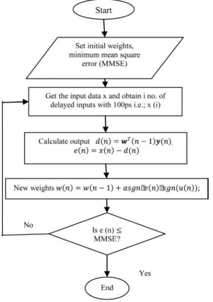
The equalizer coefficients are computed by the sign-sign least mean square (SS-LMS) method, because it de-monstrates the simplicity and robustness needed for realization in very high speed circuits [15]. The flowchart for Sign-Sign Least Mean Square (SS-LMS) algorithm shown in Figure 4 has been summarized as follows [16]:
Step 1: The very first step was to set the initial filter weights, minimum mean square error.
Step 2: After that the i no. of time delayed versions of received signal using 100 ps time delay was multip-lied with these weights and got actual output which was summation of all these terms.
[image:3.595.194.434.283.399.2]OALibJ | DOI:10.4236/oalib.1100676 4 July 2014 | Volume 1 | e676 Figure 3. A basic linear equalizer during training [13].
Figure 4. Flow chart of Sign-Sign LMS algorithm.
( )
( ) ( )
e n =u n −y n (4) where n is number of inputs, u n
( )
is desired output signal, y n( )
actual output and e n( )
is error signal.Step 4: Then the filter weights was updated using sign-sign least mean square method as given in following equation [15]:
( )
(
1)
sgn(
( )
)
sgn(
( )
)
OALibJ | DOI:10.4236/oalib.1100676 5 July 2014 | Volume 1 | e676 1 0 2 N i i α λ =
< <
∑
(6)Since λi is the 𝑖𝑖th eigenvalue of the covariance matrix RNN.
Step 5: This procedure was repeated until the limit of minimum mean square error was achieved.
6. Recursive Least Square Algorithm
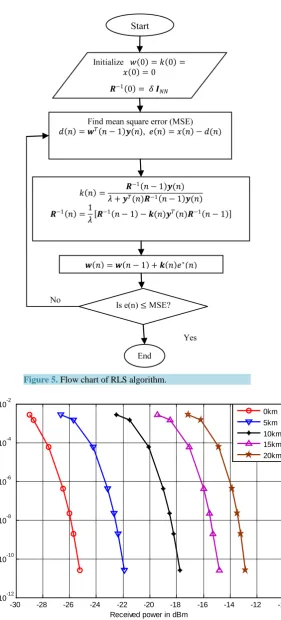
The convergence rate of the gradient based Least mean square algorithm is very slow, in order to achieve faster convergence, complex algorithms which involve additional parameters to control the adaptation rate are used. Recursive least square algorithm is based on a least squares approach, which significantly improves the conver-gence of adaptive equalizers [17] [18]. The flowchart for RLS algorithm shown in Figure 5 has been summa-rized as follows [13]:
Step 1: First of all w
( )
0 =k( )
0 =x( )
0 =0 and R−1( )
0 =δ
INN, was initialized. where INN is an N×N identity matrix, and δ is a large positive constant.Step 2: Then value of d n
( )
was calculated using the following equation [16]:( )
T(
) ( )
1
d n =w n− y n (7) where wT
(
n−1)
is the transpose of previous weights and y( )
n are the actual outputs.Step 3: After that value of error signal e n
( )
was calculated using following equation [16]:( )
( )
( )
e n =x n −d n (8) where x n
( )
is the desired output.Step 4: Then value of k n
( )
and R−1( )
n were calculated using following equations [19]:( )
T( )
1(
1(
) ( )
) ( )
1
1
n n
k n
n n n
λ − − − = + − R y
y R y (9)
( )
(
) ( ) ( )
(
)
1 n 1 1 n 1 n T n 1 n 1
λ
− = − − − − −
R R k y R (10) where λ is weighting coefficient.
Step 5: By using the value of these above equations new weights were calculated given by [19]:
( )
n =(
n− +1) ( ) ( )
n e n∗w w k (11) Step 6: This weight update procedure was repeated until the value of mean square error was less than or equal to minimum MSE value.
The λ is the weighing coefficient that can change the performance of the equalizer. Usually this factor vary from 0.8< <λ 1. The value of λ has no influence on the rate of convergence, but does determine the tracking ability of the RLS equalizers. The smaller is the value of λ, the better the tacking ability of the equalizer. However if λ is too small, the equalizer will be unstable [20].
7. Results and Discussions
The results obtained with Sign-Sign Least Mean Square and Recursive Least Square algorithm by performing various experiments, have been summarized in Figures 6-9.
Figure 6 shows the Bit error rate (BER) versus Received power in dBm without EDC for different values of fiber length at typical dispersion value of 17 ps/nm-km. The required value of received power at the input of optical fiber receiver is −25.7 dBm, −22.36 dBm, −18.23 dBm, −15.28 dBm, and −13.24 dBm for fiber length of 0 km, 5 km, 10 km, 15 km and 20 km respectively to maintain bit error rate of 1.974 10× −9. The percentage in-crease in required received power is 14.94, 40.97, 68.19 and 94.11 without EDC for fiber length 5 km, 10 km, 15 km and 20 km respectively.
OALibJ | DOI:10.4236/oalib.1100676 6 July 2014 | Volume 1 | e676 Figure 5. Flow chart of RLS algorithm.
Figure 6. BER versus Received power in dBm without EDC for different values of fiber length at typical dispersion value of 17 ps/nm-km.
-30 -28 -26 -24 -22 -20 -18 -16 -14 -12 -10
10-12 10-10 10-8 10-6 10-4 10-2
Received power in dBm
BER
[image:6.595.198.430.83.446.2]OALibJ | DOI:10.4236/oalib.1100676 7 July 2014 | Volume 1 | e676 Figure 7. BER versus Received power in dBm with EDC using
SS-LMS for different values of fiber length at typical dispersion value of 17 ps/nm-km.
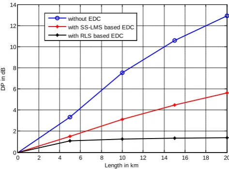
[image:7.595.195.432.83.249.2]Figure 8. BER versus Received power in dBm with EDC using RLS for different values of fiber length at typical dispersion value of 17 ps/nm-km.
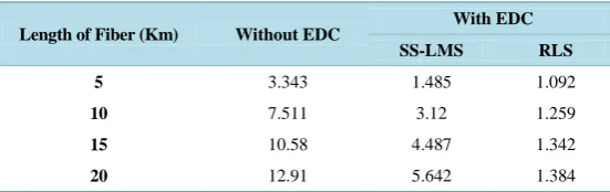
Figure 9. Dispersion penalty (DP) in dB versus fiber length in km without and with EDC using SS-LMS and RLS algorithms.
-30 -28 -26 -24 -22 -20 -18 -16 -14 -12 -10 10-12
10-10 10-8 10-6 10-4 10-2
Received power in dBm
BER
0km 5km 10km 15km 20km
-30 -29 -28 -27 -26 -25 -24 -23 10-12
10-10 10-8 10-6 10-4 10-2
Received power in dBm
BER
0km 5km 10km 15km 20km
0 2 4 6 8 10 12 14 16 18 20 0
2 4 6 8 10 12 14
Length in km
D
P
i
n dB
without EDC
[image:7.595.193.434.296.472.2] [image:7.595.194.431.520.695.2]OALibJ | DOI:10.4236/oalib.1100676 8 July 2014 | Volume 1 | e676 Table 1. Measured dispersion penalty (dB), defined at BER = 1.97 × 10⁻⁹ at
typical dispersion value of 17 ps/nm-km.
Length of Fiber (Km) Without EDC With EDC
SS-LMS RLS
5 3.343 1.485 1.092
10 7.511 3.12 1.259
15 10.58 4.487 1.342
20 12.91 5.642 1.384
fiber length of 0 km, 5 km, 10 km, 15 km and 20 km respectively to maintain bit error rate of 1.974 10× −9. The percentage increase in required received power is 6.11, 13.82, 21.16, and 27.92 with SS-LMS algorithm for fiber length 5 km, 10 km, 15 km and 20 km respectively.
Figure 8 shows the Bit error rate (BER) versus Received power in dBm with EDC using RLS for different values of fiber length at typical dispersion value of 17 ps/nm-km. The required value of received power at the input of optical fiber receiver is −25.7 dBm, −24.61 dBm, −24.44 dBm, −24.36 dBm, and −24.22 dBm for fiber length of 0 km, 5 km, 10 km, 15 km and 20 km respectively to maintain bit error rate of 1.974 10× −9. The per-centage increase in required received power is 4.43, 5.15, 5.5, and 6.11 with RLS algorithm for fiber length 5 km, 10 km, 15 km and 20 km respectively.
Figure 9 shows Dispersion penalty (DP) in dB versus fiber length in km without and with EDC using SS- LMS and RLS algorithms. Here the percentage increase in fiber length of 300, the dispersion penalty has in-creased by 286% without EDC, 279.93% with SS-LMS based EDC and 26.73% with RLS based EDC at typical value of 17 ps/nm-km. The maximum value of dispersion penalty is 12.91, 5.642 and 1.384 without EDC, with SS-LMS based EDC and with RLS algorithm based EDC at 20 km fiber length and fiber dispersion of 17 ps/nm- km. This figure shows the EDC with SS-LMS algorithm roughly doubles the transmission length and the EDC with RLS algorithm roughly ten times the transmission length for the same value of dispersion penalty.
Table 1 shows the value of dispersion penalty which is obtained without EDC and with EDC by using various algorithms at BER of 1.97 10× −9 and typical dispersion value of 17 ps/nm-km, for different value of fiber length.
Table 1 shows that for length of 20 km the value of dispersion penalty without EDC is 12.91 and dispersion penalty with EDC using SS-LMS and RLS algorithm is 5.642 and 1.384.
8. Conclusion
It has been found from this study that the performance of two algorithms is different because the convergence rate of Sign-Sign LMS algorithm depends only on single parameter but RLS algorithm convergence rate de-pends on many parameters. Sign Least Mean Square Algorithm approximately doubles the usable fiber length for a given value of dispersion penalty, and this algorithm is simplest and requires less memory to store equaliz-er coefficients. Anothequaliz-er conclusion from this study is that the EDC using Feed-forward Equalizequaliz-er with Recur-sive Least Square algorithm approximately achieves ten times the usable fiber length for given value of disper-sion penalty means achieves faster convergence, but this algorithm is very complex and requires more memory because matrix inversion is performed in this algorithm. So, if the system cost is major factor then Sign-Sign Least Mean Square algorithm is the preferred algorithm and if usable fiber length is the major aspect then Re-cursive Least Square Algorithm is used.
References
[1] Savory, S.J. (2008) Digital Filters for Coherent Optical Receivers. Optics Express, 16, 804-817. http://dx.doi.org/10.1364/OE.16.000804
[2] Savory, S.J. (2010) Digital Coherent Optical Receivers: Algorithms and Subsystems. IEEE Journal of Selected Topics Quantum Electronics, 16, 1164-1179. http://dx.doi.org/10.1109/JSTQE.2010.2044751
[3] Lavery, D., et al. (2013) Digital Coherent Receivers for Long-Reach Optical Access Networks. Journal of Lightwave Technology, 31, 609-620. http://dx.doi.org/10.1109/JLT.2012.2224847
OALibJ | DOI:10.4236/oalib.1100676 9 July 2014 | Volume 1 | e676 tion. IEEE Photonics Technology Letters, 19, 969-971. http://dx.doi.org/10.1109/LPT.2007.898819
[5] Agrawal, G.P. (2010) Fiber-Optic Communication Systems. Wiley, New York. http://dx.doi.org/10.1002/9780470918524
[6] Davis, C.C. and Murphy, T.E. (2011) Fiber-Optic Communications. IEEE Signal Processing Magazine, 28, 150-152. http://dx.doi.org/10.1109/MSP.2011.941096
[7] Azadet, K., et al. (2002) Equalization and FEC Techniques for Optical Transceivers. IEEE Journal of Solid-State Cir- cuits, 37, 317-327. http://dx.doi.org/10.1109/4.987083
[8] Winzer, P.J., et al. (2005) 10-Gb/s Upgrade of Bidirectional CWDM Systems Using Electronic Equalization and FEC. Journal of Lightwave Technology, 1, 203-210. http://dx.doi.org/10.1109/JLT.2004.840369
[9] Štěpánek, L. (2012) Chromatic Dispersion in Optical Communications. International Journal of Modern Communica-tion Technologies & Research, 7.
[10] Agrawal, G.P. (2002) Fiber-Optics Communication Systems. 3rd Edition, John Wiley and Sons, Inc., 16. http://dx.doi.org/10.1002/0471221147
[11] Casimer, M.D., et al. (2001) Fiber Optics Essential. Journal of Fiber Optic Technology, Elsevier.
[12] Feuer, M.D., et al. (2003) Electronic Dispersion Compensation for a 10-Gb/s Link Using a Directly Modulated Laser. IEEE Photonics Technology Letters, 15, 1788-1790. http://dx.doi.org/10.1109/LPT.2003.819741
[13] Rappaport, T.S. (1996) Wireless Communications-Principles and Practice. 2nd Edition, Prentice Hall. [14] Qureshi, S.U.H. (1985) Adaptive Equalization. Proceeding of IEEE, 37, 1340-1387.
[15] Shoval, A., et al. (1995) Comparison of DC Offset Effects in Four LMS Adaptive Algorithms. IEEE Transactions on Circuits and Systems-II, 42, 176-185.
[16] Alexander, S.T. (1986) Adaptive Signal Processing. Springer-Verlag. http://dx.doi.org/10.1007/978-1-4612-4978-8 [17] Haykin, S. (1986) Adaptive Filter Theory. Prentice Hall, Englewood Cliffs.
[18] Proakis, J. (1991) Adaptive Equalization for TDMA Digital Mobile Radio. IEEE Transactions on Vehicular Technol-ogy, 40, 333-341. http://dx.doi.org/10.1109/25.289414
[19] Bierman, G.J. (1988) Factorization Method for Discrete Sequential Estimation. Academic Press, New York.
![Figure 1. The dependence of pulses overlap on transmission rate [9].](https://thumb-us.123doks.com/thumbv2/123dok_us/8082255.782648/3.595.194.434.283.399/figure-dependence-pulses-overlap-transmission-rate.webp)