An Asymmetric Block Dynamic Conditional Correlation Multivariate GARCH Model

An Asymmetric Block Dynamic

Conditional Correlation Multivariate

GARCH Model

Vargas, Gregorio A.

January 2006

An Asymmetric Block Dynamic Conditional

Correlation Multivariate GARCH Model

1

Gregorio A. Vargas III2

Received: June 2006; Revised: August, 2006

ABSTRACT

The Block DCC model for determining dynamic correlations within and between groups of financial asset returns is extended to account for asymmetric effects. Simulation results show that the Asymmetric Block DCC model is competitive in in-sample forecasting and performs better than alternative DCC models in out-of-sample forecasting of conditional correlation in the presence of asymmetric effect between blocks of asset returns. Empirical results demonstrate that the model is able to capture the asymmetries in conditional correlations of some blocks of currencies in East Asia in the turbulent years of the late 1990s.

Keywords: asymmetric effect, block dynamic conditional correlation, multivariate GARCH JEL Codes: C32, C5, G10

I. INTRODUCTION

By now, the GARCH model of Bollerslev (1986) has been extended to several classes of multivariate GARCH models (see Bauwens, Laurent and Rombouts (2006)). GARCH itself has come a long way since Robert Engle’s (1982) pioneering paper on the ARCH. Multivariate GARCH (MGARCH) research focuses on ways of simplifying the variance-covariance matrix where the number of parameters to be estimated explodes for higher dimensions making estimation costly and computationally intractable. The approaches to simplify the estimation of the parameters of the variance-covariance matrix are now well-developed although suggestions have been made to come up with models that account for economic theory as a basis for simplifying this matrix, Diebold (2004).

It is widely held in financial econometrics that the returns of financial assets move together. The behavior of returns can be investigated using volatility models. Although models of MGARCH have accounted for the stylized fact that returns of similar assets move together there are other salient features of financial assets that need to be considered. Dissimilar assets have varying degrees of return correlation and one set of assets serves as a leading source of volatility for other sets of assets. Conditional correlation research has gained momentum only in recent years but its unconditional counterpart is the most common input to models being used by a typical investor.

The differences in types of financial assets result in certain groups of asset returns to be more correlated with each other than they are relative to others (see Kroner and Ng (1998), Billio,

1

This paper was supported by the Statistical Research and Training Center under its Thesis Fellowship Program for the year 2006.

2

Caporin and Gobbo (2003)). Examples of these groups are the property, food and beverage, energy, banking and finance, mining sectors in a stock market. Stock price returns within each sector are highly correlated with each other and the degree and direction of correlations between sectors are known to vary. It has been observed that the impact of bad news on stock price return correlations is asymmetric between small and large firms. It is greater on small firms when bad news occur with large firms but not vice-versa, Kroner and Ng (1998). This is important in asset allocation where investors decide what proportion of different types of instruments should comprise their portfolio to lower the risk of their overall holdings while at the same time maximize their returns. This asymmetric behavior when applied to asset allocation modeling leads to economically significant gains in an investor’s portfolio according to Patton (2004).

Asymmetric effect occurs when unexpected downward movements in the price of an asset raise the conditional volatility of returns more than when there are unexpected upward movements (see Nelson (1991) and Engle and Ng (1993)). The asymmetric effect was confirmed by empirical investigations of French, Schwert and Stambaugh (1987), Schwert (1990) and Nelson (1991) among others. In the stock market studies, Erb, Harvey and Viskanta (1994), Ang and Chen (2001), Longin and Solnik (2001) have shown that there is greater dependence between returns during market downturns.

Asymmetric effect in groups or blocks of financial asset returns were also observed by Lo and MacKinlay (1990) and Conrad, Gultekin and Kaul (1991). The lead-lag effect in portfolio returns by Lo and MacKinlay (1990) states that small firm portfolio returns lag large firm portfolio returns but not the other way around while the volatility spill-over hypothesis by Conrad, Gultekin and Kaul (1991) claims that volatility spills over large to medium and medium to small firms but not in the opposite way. Milunovich (2003) confirmed these asymmetric behaviors in stock prices of blocks of small, medium and large firms using a structural MGARCH model.

In the study of worldwide linkages in the dynamics of volatility and correlations of bonds and equity markets Capiello, Engle and Sheppard (2003) showed that there were strong asymmetries in conditional volatility of equity index returns while bond index returns have little evidence of this behavior. Cappiello, Engle and Sheppard (2003) estimated the correlations of stock and bond indices of four major regions assuming the same dynamic condition for the correlations. On the other hand, Billio, Caporin and Gobbo (2003) introduced Block Dynamic Conditional Correlation (BDCC) which assumes different dynamic condition for correlation of assets within a certain block of assets. But Billo, Caporin and Gobbo’s (2003) BDCC does not account for asymmetries between blocks while the Asymmetric DCC (ADCC) model of Cappiello, Engle and Sheppard (2003) does not consider the asymmetric correlations between blocks of assets per se. Cappiello, Engle and Sheppard (2003) only took the average dynamic correlations of individual indices to represent regional dynamic conditional correlations.

IV the model is applied to East Asian currency returns and in the last section is the conclusion.

II. THE MODEL

This paper proposes a new model called Asymmetric Block Dynamic Conditional Correlation (ABDCC) MGARCH. A missing element in the DCC literature is the asymmetric effect in the conditional correlation between blocks of asset returns and this is the contribution of ABDCC. Actually, Cajigas and Urga (2005) have accounted for this kind of asymmetry in their Asymmetric Generalized DCC (AGDCC) but theirs is a special case of the proposed model. DCCs belong to the nonlinear class of MGARCH models that aims to reduce the dimensionality of the conditional variance-covariance matrix, H_t, by specifying the conditional correlation matrix. Bauwens, Laurent and Rombouts (2006) provide the most recent and comprehensive survey of the different classes of MGARCH models.

The general representation of the MGARCH model is

t t t

y =µ +ε

t t t H z

2 / 1 =

ε where z_t~N(0,I) (1)

1

|ℑt₋ t

ε ~N(0,Ht)

where y_t is the N×1 vector of asset returns and ℑ_t−1 is a sigma algebra of information up to time t−1. Without loss of generality µ_t is assumed to be zero. The ABDCC model has the following specification for the N×N conditional variance-covariance matrixH_t:

(

ijt iit jjt

)

t t t

t DRD h h

H = = ρ _{, , ,} (2)

as in Engle’s (2002) DCC model where D_t =diag

(

h₁₁1/_,2_t h_NN1/2_,t

)

. R_t =Q_t*−1Q_tQ_t*−1 is the

N

N× matrix of dynamic conditional correlation driven by the evolution process Q_t =

( )

q_ij,t

where Qt diag

(

qii,t

)

* ₌

. The ABDCC has the following specification for Qt:

(

( ) ( ) ( )

)

( ) ( _t* _t*') ( ) _t ( ) ( _{t t}')

t Q L Q L Q L N L L Q L nn

Q = −α −β −η +α ε ε +β +η (3)

where indicates the Hadamard product, Q =E[ε_t*ε_t*'] with sample equivalent

T Q

T

t t t

= = 1

* *

'

ˆ ε ε _{that serves as estimator of Q,} *

t

ε ~N(0,R_t) is an N×1 vector of residuals

standardized by their conditional standard deviation, N =E

[

n_tn_t'

]

with sample equivalent

T n n N

T

t t t

= = 1

'

ˆ _{that serves as estimator of N,} * *

]

[ _{t t}

t I

) (L

β and η(L) are N×N parameter matrices where the N asset returns series are grouped in w sets of m₁,m₂,...,m_w -dimensional vectors and

= = q i i iL L 1 ) ( α α , = = p j j jL L 1 ) ( β β , = = r k k kL L 1 ) ( η η .

Furthermore, αi, βj and ηk have the following structure

= )' ( ) ( )' ( ) ( )' ( ) ( )' ( ) ( )' ( ) ( )' ( ) ( )' ( ) ( )' ( ) ( )' ( ) ( , 2 2 , 1 1 , 2 2 , 2 2 22 , 1 2 21 , 1 1 , 2 1 12 , 1 1 11 , w w ww i w w i w w i w w i i i w w i i i i m i m i m i m i m i m i m i m i m i m i m i m i m i m i m i m i m i m i α α α α α α α α α α = )' ( ) ( )' ( ) ( )' ( ) ( )' ( ) ( )' ( ) ( )' ( ) ( )' ( ) ( )' ( ) ( )' ( ) ( , 2 2 , 1 1 , 2 2 , 2 2 22 , 1 2 21 , 1 1 , 2 1 12 , 1 1 11 , w w ww j w w j w w j w w j j j w w j j j j m i m i m i m i m i m i m i m i m i m i m i m i m i m i m i m i m i m i β β β β β β β β β β = )' ( ) ( )' ( ) ( )' ( ) ( )' ( ) ( )' ( ) ( )' ( ) ( )' ( ) ( )' ( ) ( )' ( ) ( , 2 2 , 1 1 , 2 2 , 2 2 22 , 1 2 21 , 1 1 , 2 1 12 , 1 1 11 , w w ww k w w k w w k w w k k k w w k k k k m i m i m i m i m i m i m i m i m i m i m i m i m i m i m i m i m i m i η η η η η η η η η η

where i(m_g) is a column vector of ones with dimension m_g and g ={1,2,...,w}. i

L is the

time lag of order i.

Parameter estimation of the ABDCC model invokes the concept of variance targeting introduced by Engle and Mezrich (1996). Variance targeting assumes that in the long run the

t

Q approaches the sample variance-covariance matrix. In order to ensure that the estimation is conducted within a valid parameter space, ABDCC must be specified by maintaining the positive definiteness of the conditional correlation matrix, R_t. This can be done if Q_t is

positive definite. The following conditions ensure the positive definiteness of Q_t:

1.

(

Q −α(L) Q −β(L) Q −η(L) N

)

must be positive definite;

2. α(L)

(

εt*εt*'

)

must be positive semidefinite;

3. β(L) Q_t must be positive definite; and

In the optimization, these conditions make the location of the maximum of the likelihood function difficult. According to Engle and Sheppard (2001), a sufficient but not necessary condition for Q_t to be positive definite is for all the parameters to be positive; and, a

minimum condition to ensure the positive definiteness of Q_t is for the first condition to be satisfied as shown by Engle and Mezrich (1996).

An alternative model of ABDCC is

Q_t =

(

I−α(L)−β(L)−η(L)

)

Q +α(L) (ε_t*ε_t*')+β(L) Q_t +η(L) (n_tn_t'), (4) but this specification no longer satisfies variance targeting. Conditions 1 to 4 above still apply to this alternative model where in the first condition

(

Q −α(L) Q −β(L) Q −η(L) N

)

is replaced by

(

I−α(L)−β(L)−η(L)

)

Q .

The ABDCC, Eq. (3), regresses to the following models:

1. Engle’s (2002) DCC if the elements of α(L), β(L) and η(L) have αij =a in α(L), b

ij =

β in β(L), andη(L)=0, for all i,j∈

{

1,...,N

}

; 2. Billio, Caporin and Gobbo’s (2003) BDCC if η(L)=0;

3. Cappiello, Engle and Sheppard’s (2003) ADCC if the elements of α(L), β(L) and

) (L

η have αij =

( )

a 2 in α(L),

( )

2

b ij =

β in β(L), and ηij =

( )

g 2 in η(L), for all

{

N

}

j

i, ∈ 1,..., ;

4. Cajigas and Urga’s (2005) AGDCC, if the elements of α(L), β(L) and η(L) have

2

ii ii =a

α and α_ij =a_iia_jj in α(L), β_ii =b_ii2 and β_ij =b_iib_jj in β(L), η_ii =g_ii2 and

jj ii ij =g g

η in η(L), for all i,j∈

{

1,...,N

}

where i≠ j.

for time lag of order 1. These can be easily generalized to higher orders of time lag. While the alternative ABDCC, Eq. (4), regresses to Cajigas and Urga’s (2005) alternative AGDCC if the same conditions in No.4 are satisfied.

The likelihood function of ABDCC is derived under the assumption that the underlying distribution of the vector of returns is multivariate normal. Limited information maximum likelihood (LIML) is utilized here. In a two-stage LIML parameter estimation procedure the set of parameters is divided into two. The likelihood function is maximized with respect to the first set of parameters then the parameter estimates of the first set serve as inputs to the second stage where the next set of parameters are then estimated. The likelihood function of the model is

(

)

Π =

−

− =

' 2 1

1

1

2 1

2 1 )

| ,

( ytHt yt

t N T

t

t e

H y

L

π ϕ

ϑ . (5)

( )

(

)

= − + + − = T t t t t t

t N H y H y

y L 1 1 ' log 2 log 2 1 ) | , (

log ϑ ϕ π

( )

(

)

= − − − + + + − = T t t t t t t t

t D y D R D y

R N 1 1 1 1 ' log 2 log 2 log 2 1

π (6)

where H_t =D_tR_tD_t andD_t =diag

(

h₁₁1/_,2_t h1_NN/2_,t

)

. As shown by Engle and Sheppard (2001), if

t

R is assumed to be an identity matrix in the first stage estimation,

( )

(

)

= − − − + + + − = T t t t N t t t N

t N I D y D I D y

y L 1 1 1 1 ' log 2 log 2 log 2 1 ) | (

log ϑ π (7)

ϑˆ=argmax[logL(ϑ|yt)] (8)

turns out to be the univariate estimation of the individual GARCH models of asset returns of

t

y . The second stage estimation will have

( )

(

)

= − − − + + + − = T t t t t t t t t

t N R D y D R D y

y L 1 1 1 1 _ˆ ˆ ' ˆ log 2 log 2 log 2 1 ) , ˆ | (

log ϕ ϑ π (9)

where ε_t*=Dˆ_t−1y_t. And since R_t =Q_t*−1Q_tQ_t*−1 where Q_t* =diag

(

q_iit

)

( )

(

)

= − − − − − _{+ +} + − = T t t t t t t t t t t

t N Q QQ D Q QQ

y L 1 * 1 1 * 1 * * 1 * 1 * ) ( ' ˆ log 2 log 2 log 2 1 ) , ˆ | (

log ϕ ϑ π ε ε .

Excluding the constant terms in the loglikelihood function we have

(

)

= − − − − − ₊ − = T t t t t t t t t t

t Q QQ Q QQ

y L 1 * 1 1 * 1 * * 1 * 1 * ) ( ' log 2 1 ) , ˆ | ( '

log ϕ ϑ ε ε (10)

ϕˆ =argmax[logL'(ϕ|ϑˆ,y_t)]. (11)

Expanding the 2nd stage loglikelihood function

) , ˆ | ( '

logL ϕ ϑ y_t (12)

(

)

(

)

{

= − − _{− − − + + +} − = T t t t t t t t

t Q L Q L Q L N L L Q L nn Q

Q 1 1 * * * 1 * ) ' ( ) ( ) ( ) ' ( ) ( ) ( ) ( ) ( log 2 1 η β ε ε α η β α

(

)

(

)

(

*1 * * *1

)

1 *

}

*' ) ' ( ) ( ) ( ) ' ( ) ( ) ( ) ( )

( _{t t t t t t t}

t

t Q Q α L Q β L Q η L N α L ε ε β L Q η L nn Q ε

ε − − −

+ + + − − − +

III. SIMULATION RESULTS

Monte Carlo simulations were conducted to determine the consistency of the MLE estimator as the sample size is increased for the ABDCC in the case of a 4-dimensional vector return series, partitioned into two 2-dimensional vectors where lag orders q, p and r of L are all equal to 1 or ABDCC(2,2;1,1,1). The general notation of the model is

(

m , ,m_w;p,q,r

)

ABDCC ₁ . Three cases were considered: nonpersistent-nonpersistent, persistent-nonpersistent and persistent-persistent blocks of volatility series where each block consists of two series. A GARCH(1,1) process, hii_,t =ω₁+α₁εi2_,t₋₁+β₁hii_,t₋₁, is considered persistent if α₁+β₁ ≥0.80, the parameters α₁ and β₁ are the impact and persistence of the process. Similarly, the evolution process, Qt, of the conditional correlation consists of

impact, persistence and asymmetric effect parameters αij, βij and ηij, respectively. Conditional correlation is considered persistent within a block if α_ii +β_ii ≥0.80 and between blocks if α_ij +β_ij ≥0.80. The specifications of the model are given below.

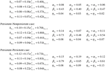
Nonpersistent-Nonpersistent case: 1 , 44 2 1 , 4 , 44 1 , 33 2 1 , 3 , 33 1 , 22 2 1 , 2 , 22 1 , 11 2 1 , 1 , 11 42 . 0 07 . 0 11 . 0 37 . 0 08 . 0 08 . 0 45 . 0 12 . 0 08 . 0 40 . 0 10 . 0 07 . 0 − − − − − − − − + + = + + = + + = + + = t t t t t t t t t t t t h h h h h h h h ε ε ε ε 04 . 0 43 . 0 08 . 0 11 11 11 = = = η β α 03 . 0 40 . 0 05 . 0 22 22 22 = = = η β α 02 . 0 47 . 0 06 . 0 21 12 21 12 21 12 = = = = = = η η β β α α Persistent-Nonpersistent case: 1 , 44 2 1 , 4 , 44 1 , 33 2 1 , 3 , 33 1 , 22 2 1 , 2 , 22 1 , 11 2 1 , 1 , 11 51 . 0 04 . 0 09 . 0 44 . 0 09 . 0 07 . 0 80 . 0 12 . 0 12 . 0 70 . 0 15 . 0 10 . 0 − − − − − − − − + + = + + = + + = + + = t t t t t t t t t t t t h h h h h h h h ε ε ε ε 08 . 0 73 . 0 14 . 0 11 11 11 = = = η β α 04 . 0 48 . 0 07 . 0 22 22 22 = = = η β α 07 . 0 54 . 0 11 . 0 21 12 21 12 21 12 = = = = = = η η β β α α Persistent-Persistent case: 1 , 44 2 1 , 4 , 44 1 , 33 2 1 , 3 , 33 1 , 22 2 1 , 2 , 22 1 , 11 2 1 , 1 , 11 64 . 0 22 . 0 08 . 0 67 . 0 20 . 0 09 . 0 81 . 0 14 . 0 11 . 0 73 . 0 17 . 0 12 . 0 − − − − − − − − + + = + + = + + = + + = t t t t t t t t t t t t h h h h h h h h ε ε ε ε 08 . 0 79 . 0 15 . 0 11 11 11 = = = η β α 09 . 0 65 . 0 19 . 0 22 22 22 = = = η β α 13 . 0 61 . 0 12 . 0 21 12 21 12 21 12 = = = = = = η η β β α α

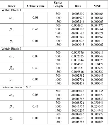
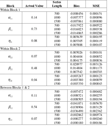
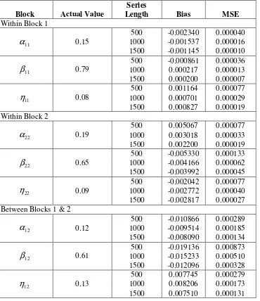
[image:8.595.70.516.347.651.2]

condition for the evolution process, Qt, to remain positive definite. As the sample size is increased, the MSE dropped for all the parameters in all cases considered and so confirms the consistency of the maximum likelihood estimator for the model.

In order to assess how well the ABDCC model performs in in-sample and out-of-sample forecasting of conditional correlation between blocks of asset returns, in the absence and presence of asymmetric effects within and between conditional correlation of blocks, its performance vis-à-vis the other dynamic conditional correlations models DCC, BDCC, ADCC and AGDCC is compared. Below are specifications for three main cases: Case A nonpersistent-nonpersistent, Case B persistent-nonpersistent and Case C persistent-persistent conditional correlations between blocks of assets for a series of 1,000 observations. There were nine cases considered in these simulations and for each 500 Monte Carlo runs were conducted. Cases 1, 2 and 3 consists of cases A, B and C, respectively, but with zero asymmetric effects, that is, η₁₁ =η₂₂ =η₁₂ =0. Cases 4, 5 and 6 follow the exact specifications of A, B and C which have small between block asymmetric effects, η₁₂’s. While cases 7, 8 and 9, on the other hand, have the same specification as A, B and C but with larger η₁₂’s of 0.12, 0.15 and 0.15, respectively.

Case A: 1 , 11 2 1 , 1 ,

11t =0.08+0.12 t− +0.55h t−

h ε 1 , 22 2 1 , 2 ,

22t =0.11+0.10 t− +0.59h t−

h ε 1 , 33 2 1 , 3 ,

33t =0.15+0.08 t− +0.64h t−

h ε 1 , 44 2 1 , 4 ,

44t =0.12+0.11 t− +0.52h t−

h ε 04 . 0 51 . 0 07 . 0 11 11 11 = = = η β α 04 . 0 58 . 0 06 . 0 22 22 22 = = = η β α 03 . 0 45 . 0 04 . 0 21 12 21 12 21 12 = = = = = = η η β β α α Case B: 1 , 11 2 1 , 1 ,

11t =0.05+0.05 t− +0.80h t−

h ε 1 , 22 2 1 , 2 ,

22t =0.10+0.07 t− +0.75h t−

h ε 1 , 33 2 1 , 3 ,

33t =0.30+0.20 t− +0.55h t−

h ε 1 , 44 2 1 , 4 ,

44t =0.40+0.17 t− +0.60h t−

Case C:

1 , 11 2

1 , 1 ,

11t =0.05+0.06 t− +0.90h t−

h ε

1 , 22 2

1 , 2 ,

22t =0.10+0.08 t− +0.85h t−

h ε

1 , 33 2

1 , 3 ,

33t =0.08+0.20 t− +0.68h t−

h ε

1 , 44 2

1 , 4 ,

44t =0.11+0.17 t− +0.72h t−

h ε

07 . 0

82 . 0

05 . 0

11 11 11

= = =

η β α

08 . 0

65 . 0

15 . 0

22 22 22

= = =

η β α

06 . 0

55 . 0

05 . 0

21 12

21 12

21 12

= =

= =

= =

η η

β β

α α

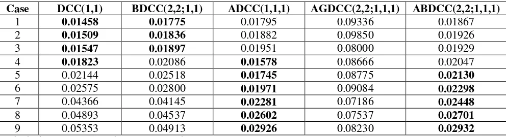
Table 2 shows the in-sample forecast performance of the different models in capturing simulated conditional correlations between two blocks of asset returns. The results show that the ADCC of Cappiello, Engle and Sheppard (2003) outperformed all the other DCC models for cases 4 to 9 in terms of the lowest average root mean squared error (RMSE) criterion in forecasting each of the 500 generated series. ADCC is best in in-sampling forecast performance for those with persistent and nonpersistent conditional correlations with small and large asymmetric effects. The ABDCC follows next for cases 5 to 9. However, the simple DCC is competitive compared to the other models with regard to nonpersistent blocks with small asymmetric effects, as seen in case 4; and it outperforms more parameterized models in nonpersistent and persistent cases without asymmetric effects as evidenced by cases 1 to 3.

For out-of-sample forecast evaluation, 500 Monte Carlo runs of 1,200 series lengths of between block conditional correlations were generated for the nine cases. The last 200 observations serve as the hold-out sample that all the models will forecast 200-step-ahead out-of-sample. Table 3 presents the average mean squared errors (MSEs) for the 500 forecast series of each of the model for each case. The DCC and BDCC models dominate those cases without asymmetric effects, cases 1 to 3; and, these can compete fairly with the others for the case of nonpersistent-nonpersistent and persistent-persistent blocks with small asymmetric effects, respectively, as seen in cases 4 and 6. But clearly, in the presence of a persistent block or blocks with small and large asymmetric effects ABDCC outperforms the rest with ADCC coming in next. These results lend support to the ABDCC model as the model of choice in out-of-sample forecasting of persistent conditional correlation between blocks of asset returns with asymmetric effects. This behavior is widely observed in portfolios of stocks providing a venue for practical application of ABDCC in asset allocation models.

model compared to BDCC and ABDCC for cases 2 and 4, respectively. While the BDCC performed 90% of the time better than DCC in case 1 but did poorly for case 3 with respect to ABDCC at 65%. The ABDCC edged out ADCC in cases 5 and 7 to 9 by 83% to 97% of the time, while it did not do as well with BDCC at 73% in case 6.

The DM and MDM tests of forecast accuracy confirmed that, in general, when persistence of conditional correlation and asymmetric effect exist within and between blocks of asset returns the ABDCC model is expected to perform better than the rest in out-of-sample forecasting. At the same time, the test results favor the parsimonious DCC and also the BDCC in cases where asymmetric effect is absent. This is expected since DCC and BDCC models assume symmetry in the conditional correlations.

IV. APPLICATION TO EAST ASIAN FOREX RETURNS

The data was derived from FXHistory in oanda.com. These are 1,279 daily average exchange rates with respect to the U.S. dollar from 1996 to 2000 of the Philippine peso (PHP), Thailand baht (THB), Malaysian ringgit (MYR), Singapore dollar (SGD), Hong Kong dollar (HKD) and China yuan (CNY). Adjustments have been made to account for holidays. An ABDCC(2,2;1,1,1) was used to model the following blocks: PHP-THB, MYR-SGD and HKD-CNY. The Philippine peso and Thailand baht are considered as a block because these two economies are regarded as twins in the ASEAN. On the other hand, Malaysian ringgit and Singaporean dollar are in another block given that these two economies are relatively larger compared to Philippines and Thailand. Hong Kong dollar and Chinese yuan belong to a block for these two economies are reasonably linked since Hong Kong became a special administrative region of China in July of 1997. Asset return here is defined as the negative of the difference in daily logarithmic forex rate.

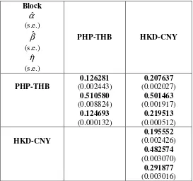
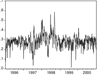
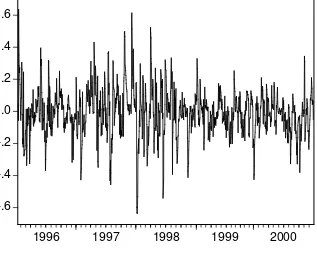
Tables 5, 6 and 7 show the conditional correlations of the blocks of currencies. All the parameters are significant at the 0.05 level except for the asymmetric effect parameter between the PHP-THB and MYR-SGD blocks as shown in Table 5. This implies that there is no significant asymmetric correlation in the volatilities of the peso-baht and ringgit-SG dollar although the conditional correlations are highly persistent between these two blocks. Asymmetry in conditional correlations is present for these two blocks when compared with the HK dollar-yuan block as presented in Tables 6 and 7. Table 7 further shows that the correlation of volatility is persistent between HK dollar-yuan and ringgit-SG dollar owing largely to the level of development and relative stability of the financial markets in Hong Kong and Singapore while HK dollar-yuan and peso-baht correlation of volatility are not as persistent. There is also a higher asymmetry in the conditional correlation of HK dollar-yuan and peso-baht.

To determine the conditional correlation between blocks, the estimated conditional variances,

t ij

the same time, there was a sharp rise in the conditional correlation of the two blocks during the 1997-98 Asian Financial Crisis. The drop in the conditional correlation occurred in September of 1998 when Malaysia imposed capital controls to discourage speculators against its currency. In Figures 2 and 3, the conditional correlations of peso-baht and ringgit-SG dollar against HK dollar-yuan is fluctuating around zero which indicate periods of positive and negative conditional correlations. But in Figure 3, the 1997-98 period resulted in higher volatility of the conditional correlation between ringgit-SG dollar and HK dollar-yuan and this volatility in conditional correlation relatively mellowed after 1998 when the ringgit exchange rate was pegged and the SG-dollar has stabilized. This is dissimilar to the pattern between peso-baht and HK dollar-yuan where the relatively stable exchange rates of the HK dollar and the yuan are fluctuating similarly across the period against the peso-baht.

The significant asymmetries of the ASEAN blocks with respect to the HK dollar-yuan block may be explained by the relatively stable movement of these two currencies compared to their ASEAN counterparts in the period considered. Hong Kong operates a form of currency board system which composes a pegged exchange rate against the U.S. dollar. The Chinese yuan is also pegged to a tight band since 1994. It follows that whatever pressure to depreciation on non-pegged currencies will not impact the pegged ones. And this is evident in the asymmetries that are observed here with respect to the HKD-CNY block. The insignificant asymmetry between the ASEAN blocks implies that although the correlation of the volatilities of the peso-baht and the ringgit-SG dollar is persistent there is no asymmetric effect in the dynamic conditional correlation of the returns between the two blocks.

V. CONCLUSION

The Asymmetric Block Dynamic Conditional Correlation model, a new model which extends the Block DCC of Billio, Caporin and Gobbo (2003), introduces the asymmetric effect in the evolution process between blocks of asset returns. The two-stage maximum likelihood estimation procedure utilizing the limited information maximum likelihood approach is shown to be consistent in estimating the parameters of the ABDCC model. Furthermore, simulation results support the ABDCC as a better model compared to other DCCs in out-of-sample forecasting of conditional correlations in the presence of asymmetric effect in dynamic conditional correlation between blocks of asset returns.

[image:13.595.72.444.147.576.2]

Table 1.1. Monte Carlo Simulation Results for Varying Sample Sizes of ABDCC(2,2;1,1,1) Model: Nonpersistent-Nonpersistent Blocks

Block Actual Value

Series

Length Bias MSE

Within Block 1

500 -0.003809 0.000166

1000 -0.004972 0.000084

11

α 0.08

1500 -0.005246 0.000065

500 0.004801 0.004376

1000 -0.001105 0.001664

11

β 0.43

1500 -0.005583 0.001024

500 -0.000749 0.000262

1000 -0.000026 0.000110

11

η 0.04

1500 -0.000043 0.000067

Within Block 2

500 0.003376 0.000114

1000 0.002025 0.000047

22

α 0.05

1500 0.001844 0.000026

500 0.054681 0.010422

1000 0.031651 0.003922

22

β 0.40

1500 0.019816 0.002329

500 -0.002382 0.000143

1000 -0.002701 0.000069

22

η 0.03

1500 -0.002479 0.000045

Between Blocks 1 & 2

500 -0.003043 0.001135

1000 -0.004683 0.000529

12

α 0.06

1500 -0.004768 0.000332

500 -0.068321 0.050844

1000 -0.043553 0.024045

12

β 0.47

1500 -0.030205 0.014946

500 -0.007086 0.001877

1000 -0.004606 0.000804

12

η 0.02

[image:14.595.76.448.121.549.2]

Table 1.2. Monte Carlo Simulation Results for Varying Sample Sizes of ABDCC(2,2;1,1,1) Model: Persistent-Nonpersistent Blocks

Block Actual Value

Series

Length Bias MSE

Within Block 1

500 -0.008456 0.000151

1000 -0.007377 0.000096

11

α 0.14

1500 -0.007061 0.000080

500 -0.017922 0.000522

1000 -0.016023 0.000338

11

β 0.73

1500 -0.014865 0.000286

500 0.005639 0.000195

1000 0.005305 0.000119

11

η 0.08

1500 0.005888 0.000107

Within Block 2

500 0.005026 0.000101

1000 0.004404 0.000052

22

α 0.07

1500 0.004175 0.000036

500 0.028977 0.003126

1000 0.014804 0.001173

22

β 0.48

1500 0.007542 0.000703

500 -0.003247 0.000123

1000 -0.003380 0.000059

22

η 0.04

1500 -0.003330 0.000043

Between Blocks 1 & 2

500 -0.007472 0.000482

1000 -0.008521 0.000255

12

α 0.11

1500 -0.008505 0.000194

500 -0.041871 0.005670

1000 -0.038906 0.003129

12

β 0.54

1500 -0.036490 0.002362

500 -0.002862 0.000574

1000 -0.000277 0.000260

12

η 0.07

[image:15.595.76.446.121.549.2]

Table 1.3. Monte Carlo Simulation Results for Varying Sample Sizes of ABDCC(2,2;1,1,1) Model: Persistent-Persistent Blocks

Block Actual Value

Series

Length Bias MSE

Within Block 1

500 -0.002340 0.000040

1000 -0.001537 0.000016

11

α 0.15

1500 -0.001145 0.000010

500 -0.000861 0.000036

1000 0.000217 0.000013

11

β 0.79

1500 0.000200 0.000007

500 0.001164 0.000077

1000 0.000701 0.000029

11

η 0.08

1500 0.000827 0.000019

Within Block 2

500 0.005067 0.000077

1000 0.003018 0.000033

22

α 0.19

1500 0.002200 0.000019

500 -0.005330 0.000133

1000 -0.004166 0.000062

22

β 0.65

1500 -0.003992 0.000045

500 -0.002042 0.000077

1000 -0.002772 0.000040

22

η 0.09

1500 -0.002817 0.000027

Between Blocks 1 & 2

500 -0.010866 0.000289

1000 -0.009514 0.000185

12

α 0.12

1500 -0.008090 0.000134

500 -0.019136 0.000873

1000 -0.015233 0.000510

12

β 0.61

1500 -0.012096 0.000328

500 0.007745 0.000279

1000 0.008206 0.000173

12

η 0.13

[image:16.595.70.566.120.255.2]

Table 2. Average RMSEs of the Different DCC Models in 500 Monte Carlo Simulations of In-Sample Forecasts in Estimating Simulated Block Dynamic Conditional Correlations

Case DCC(1,1) BDCC(2,2;1,1) ADCC(1,1,1) AGDCC(2,2;1,1,1) ABDCC(2,2;1,1,1)

1 0.01458 0.01775 0.01795 0.09336 0.01867

2 0.01509 0.01836 0.01882 0.09850 0.01926

3 0.01547 0.01897 0.01951 0.08000 0.01929

4 0.01823 0.02086 0.01578 0.08666 0.02047

5 0.02144 0.02518 0.01745 0.08775 0.02130

6 0.02575 0.02800 0.01971 0.09084 0.02298

7 0.04366 0.04145 0.02281 0.07186 0.02448

8 0.04893 0.04537 0.02602 0.07537 0.02701

9 0.05353 0.04913 0.02926 0.08230 0.02932

[image:16.595.69.569.331.465.2]

Highlighted Average RMSEs are the two lowest in each case.

Table 3. Average MSEs of the Different DCC Models in 500 Monte Carlo Simulations of 200-Step-Ahead Out-of-Sample Forecasts in Estimating Simulated Block Dynamic Conditional Correlations

Case DCC(1,1) BDCC(2,2;1,1) ADCC(1,1,1) AGDCC(2,2;1,1,1) ABDCC(2,2;1,1,1)

1 0.000345 0.000337 0.000514 0.004908 0.000787

2 0.000328 0.000367 0.000414 0.004156 0.000399

3 0.000469 0.000395 0.000509 0.001558 0.000413

4 0.000440 0.000506 0.000455 0.003909 0.000443

5 0.000604 0.000594 0.000478 0.002840 0.000477

6 0.001146 0.000769 0.000878 0.001138 0.000535

7 0.001968 0.001609 0.001021 0.002114 0.000596

8 0.002699 0.002067 0.001112 0.001746 0.000719

9 0.003879 0.002367 0.002071 0.002301 0.000830

Highlighted Average MSEs are the two lowest in each case.

Table 4. Proportion of H0 Rejections in the Mariano and the Modified Diebold-Mariano Tests in 500 Monte Carlo Simulations of 200-Step-Ahead Out-of-Sample Forecasts of the Top 2 Models from Table 3 in Estimating Simulated Block Dynamic Conditional Correlations

MSE Case

DCC(1,1) BDCC(2,2;1,1) ADCC(1,1,1) ABDCC(2,2;1,1,1)

DM Test

MDM Test

1 0.000345 0.000337 − − 0.898 0.900

2 0.000328 0.000367 − − 0.852 0.854

3 − 0.000395 − 0.000413 0.646 0.648

4 0.000440 − − 0.000443 0.812 0.814

5 − − 0.000478 0.000477 0.900 0.902

6 − 0.000769 − 0.000535 0.726 0.728

7 − − 0.001021 0.000596 0.966 0.968

8 − − 0.001112 0.000719 0.942 0.944

9 − − 0.002071 0.000830 0.830 0.832

[image:16.595.70.573.558.707.2]

[image:17.595.66.339.108.364.2]

Table 5. ABDCC(2,2;1,1,1) Model of PHP-THB and MYR-SGD Forex Returns

Block

αˆ (s.e.)

βˆ

(s.e.)

ηˆ (s.e.)

PHP-THB MYR-SGD

PHP-THB

0.164128 (0.002960)

0.523677 (0.003629)

0.046345 (0.003323)

0.041819 (0.000753)

0.824190 (0.002214)

0.002132 (0.003567)

MYR-SGD

0.129147 (0.001858)

0.508595 (0.004072)

0.087879 (0.002228)

All highlighted parameter estimates are significant at the 0.05 level.

Table 6. ABDCC(2,2;1,1,1) Model of PHP-THB and HKD-CNY Forex Returns

Block

αˆ (s.e.)

βˆ

(s.e.)

ηˆ (s.e.)

PHP-THB HKD-CNY

PHP-THB

0.126281 (0.002443)

0.510580 (0.008824)

0.124693 (0.000132)

0.207637 (0.002027)

0.501463 (0.001917)

0.219513 (0.000512)

HKD-CNY

0.195552 (0.002426)

0.482574 (0.003070)

0.291877 (0.003016)

[image:17.595.66.339.416.672.2]

[image:18.595.67.338.108.363.2]

Table 7. ABDCC(2,2;1,1,1) Model of HKD-CNY and MYR-SGD Forex Returns

Block

αˆ (s.e.)

βˆ

(s.e.)

ηˆ (s.e.)

HKD-CNY MYR-SGD

HKD-CNY

0.150419 (0.000233)

0.574708 (0.000624)

0.194977 (0.001349)

0.238101 (0.000199)

0.683436 (0.000378)

0.118465 (0.000325)

MYR-SGD

0.119230 (0.000485)

0.570860 (0.000473)

0.087742 (0.000376)

All highlighted parameter estimates are significant at the 0.05 level.

Figure 1. Asymmetric Block DCC of PHP-THB and MYR-SGD Blocks of Forex Returns

.0 .1 .2 .3 .4 .5 .6 .7

[image:18.595.89.405.451.703.2]

[image:19.595.88.405.122.377.2]

Figure 2. Asymmetric Block DCC of PHP-THB and HKD-CNY Blocks of Forex Returns

-.6 -.4 -.2 .0 .2 .4 .6

1996 1997 1998 1999 2000

Figure 3. Asymmetric Block DCC of HKD-CNY and MYR-SGD Blocks of Forex Returns

-.6 -.4 -.2 .0 .2 .4 .6

[image:19.595.89.406.441.696.2]

ACKNOWLEDGEMENTS

The author is very grateful to Adolfo de Guzman for enriching discussions and critical suggestions

that greatly improved this paper. Helpful comments from Russel Reyes and Jonathan Yabes in the

computing aspect have been beneficial in the simulation exercise. Thanks also to Joselito Magadia,

Welfredo Patungan, Dennis Mapa, Michael McAleer, David Dickinson, Kevin Sheppard, Xiangdong

Long and to an anonymous referee. Valuable comments are recognized from participants of the UP

School of Statistics colloquium series, the Statistical Research and Training Center (SRTC) seminar

and the Econometrics Society Australasian Meeting 2006 in Alice Springs, Australia.

References

Ang, A. and J. Chen (2001), “Asymmetric Correlations of Equity Portfolios,” Journal of Financial Economics, 63(3), 443-494.

Bauwens, L., S. Laurent and J.V.K. Rombouts (2006), “Multivariate GARCH Models: A Survey,” Journal of Applied Econometrics, 21(1), 2006.

Billio, M., M. Caporin and M. Gobbo (2003), “Block Dynamic Conditional Correlation Multivariate GARCH Models,” Working Paper 03.03, Gruppi di Ricerca Economica Teorica e Applicata, Venice.

Bollerslev, T. (1986), “Generalized Autoregressive Conditional Heteroskedasticity,” Journal of Econometrics, 31, 307-327.

Cajigas, J. and G. Urga (2005), “Dynamic Conditional Correlation Models with Asymmetric Multivariate Laplace Innovations,” Centre for Econometric Analysis, Cass Business School.

Cappiello L., R.F. Engle and K. Sheppard (2003), “Asymmetric Dynamics in the Correlations of Global Equity and Bond Returns,” Working Paper No. 204, European Central Bank.

Conrad, J., M. Gultekin and G. Kaul (1991), “Asymmetric Predictability of Conditional Variances,” Review of Financial Studies, 4, 597-622.

Diebold, F.X. (2004), “The Nobel Memorial Prize for Robert F. Engle,” Scandinavian Journal of Economics, 106, 165-185.

Diebold, F.X. and R. S. Mariano (1995), “Comparing Predictive Accuracy,” Journal of Business and Economic Statistics, 13(3), 253-263.

Engle, R.F. (2002), “Dynamic Conditional Correlation: A Simple Class of Generalized Autoregressive Conditional Heteroskedasticity Models,” Journal of Business and Economic Statistics, 20, 339-350.

Engle, R.F. and J. Mezrich (1996), “GARCH for Groups,” Risk August, 9(8), 36-40.

Engle, R.F. and V.K. Ng (1993), “Measuring and Testing the Impact of News on Volatility,” Journal of Finance, 48, 987-1008.

Engle, R.F. and K. Sheppard (2001), “Theoretical and Empirical Properties of Dynamic Conditional Correlation Multivariate GARCH,” Working Paper 8554, National Bureau of Economic Research.

Erb, C.B., C.R. Harvey and T.E. Viskanta (1994), “Forecasting International Equity Correlations,” Financial Analysts Journal, 50, 32-45.

French, K.R., G.W. Schwert and R.F. Stambaugh (1987), “Expected Stock Returns and Volatility,” Journal of Financial Economics, 19, 3-29.

Harvey, D., S. Leybourne and P. Newbold (1997), “Testing the Equality of Prediction Mean Squared Errors,” International Journal of Forecasting, 13, 281-291.

Kroner, K.F. and V. Ng (1998), “Modeling Asymmetric Comovements of Asset Returns,” Review of Financial Studies, 11, 817-844.

Lo, A. and C. MacKinlay (1990), “When are Contrarian Profits due to Stock Market Overreaction?” Review of Financial Studies, 3, 175-205.

Longin, F. and B. Solnik (2001), “Extreme Correlation of International Equity Markets,” Journal of Finance, 56(2), 646-676.

Milunovich, G.D. (2003), “Modeling Dependence Structure in Size-Sorted Portfolios: A Structural Multivariate GARCH Model,” Working Paper, School of Economics, University of New South Wales.

Nelson, D.B. (1991), “Conditional Heteroskedasticity in Asset Returns: A New Approach,” Econometrica, 59, 347-370.

Patton, A. (2004), “On the Out-of-Sample Importance of Skewness and Asymmetric

Dependence for Asset Allocation,” Journal of Financial Econometrics, 2(1), 130-168.

Schwert, G.W. (1990), “Stock Volatility and the Crash of ’87,” Review of Financial Studies, 3, 77-102.