Using Multiple Path Constraint Mobile Sinks for Energy Efficient Data Collection in Wireless Sensor Networks

Using Multiple Path-Constraint Mobile Sinks for Energy

Efficient Data Collection in Wireless Sensor Networks

P.Majal Stepa Shiny

PG Scholor,Department of Information Technology, Regional Center Anna University, Coimbatore

ABSTRACT

Data collection is a fundamental task of WSN. It aims to collect sensor readings in a sensory field through sinks for analysis and processing. Research has shown that sinks deplete most of the battery power for collecting the data than processing it. Non-uniform energy consumption causes degraded network performance and shortens network lifetime. Recently, sink mobility with limited path has been exploited to reduce and balance the energy expenditure among sensors. This paper address this issue and propose a new data collection scheme, which enhance the Maximum Amount Shortest Path (MASP) for Multiple Mobile Sinks. This scheme increases network throughput and streamlining the energy consumption by optimizing the assignment of sensor nodes to subsinks and subsinks to mobile sinks, using Genetic Algorithm. An existing two-phase communication protocol designed for single mobile sink is enhanced to support multiple mobile sinks. The proposed algorithms and protocols are validated through simulation experiments using NS2.

Keywords- Wireless Sensor Networks ( WSN), Maximum Amount Shortest Path(MASP), Mobile sink,Subsink,Direct Communication Area(DCA) ,Multihop Communication Area(MCA)

1.

INTRODUCTION

Wireless Sensor Networks (WSNs) have been widely considered as one of the most important technologies for the twenty-first century. A WSN typically consists of a large number of low-priced, low-power, and multi- functional sensor nodes that are deployed in a region of significance. These sensor nodes are small in size, but are equipped with sensors, implant microprocessors, and radio transceivers, and therefore have not only sensing capacity, but also data handling and communicating capability. They communicate over a short distance via a wireless medium and work together to complete a common task, for example, environment monitor, battlefield observation, and industrial process control. Reducing energy utilization is the most important objective in the design of a sensor network. Sensor nodes are power-driven by battery and it is often very difficult or even impossible to change or renew their batteries, it is crucial to reduce the power use of sensor nodes so that the lifetime of the sensor nodes, as well as the whole network is extended.

2.RELATED WORK

In [1],[2] the mobile sinks are fixed on vehicles or animals moving randomly to collect information that are sensed by the sensor node .It also analyses architecture to collect sensor data in sparse sensor networks. This approach exploits the presence of mobile entities (called MULEs) present in the surroundings.

MULEs accept data from the sensor in secure range, safeguard it, and drop off the data to wired access points.

In [3],[4], path constrained sink mobility is used to improve the energy efficiency in sensor networks using single hop which may be infeasible because of the limits of location and communication power. A routing protocol called MobiRoute is proposed in [7] for Wireless Sensor Networks with a path predictable mobile sink where all sensor nodes need to be aware of the movement of the mobile sink. In [3],[4],[6] various data collection problems are concerned to improve the performance of the network. In [5], path constrained sink mobility is discussed to improve the energy efficiency of multihop sensor networks using a single mobile sink. They have also contains the coding for MASP for single mobile sink. In this paper a code is developed for multiple mobile sink to increase the amount of gathered data and decrease the energy consumption.

3.SYSTEM ARCHITECTURE

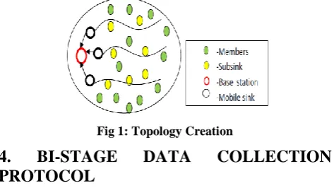
[image:1.595.306.543.516.649.2]

Based on the communication area of the mobile sinks the coverage area can be divided into two parts ,the Direct Communication Area (DCA) and Multihop Communication area (MCA).Sensor nodes that presents inside the DCA are called subsinks ,which can directly transmit data to the mobile sinks because they are close to the trajectory of mobile sinks. And the sensor nodes residing within the MCA are called members, transmit the data to the mobile sink through subsinks(sensor to subsink and subsink to mobile sink)

Fig 1: Topology Creation

4.

BI-STAGE

DATA

COLLECTION

PROTOCOL

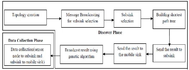
A Bi-stage data collection protocol is proposed in this chapter which includes efficient subsink discovery and data collection procedures. It consist of two main phases: Discover phase and Data Collection phase.

4

.1 Discover Phase

Step1:

In this step all the mobile sinks transmit the broadcast messages continuously. The nodes that are receiving the broadcast messages from the mobile sink are automatically selected as the subsink of the corresponding mobile sink.Then the SPT(Shortest Path Tree) is developed fot the entire network.

Step2:

In this step the subsinks send the shortest hop information collected in step 1 to their corresponding mobile sink when it passing it.This information is enough for MASP calculation.Finally Gentic algorithm (In section 6) is executed to obtain the optimized assignment between all subsink and mobile sink and all members to subsink.

Step 3:

In step 3,All the mobile sinks traverse the path again to broadcast the results of the member and subsink assignment.

4.2 Data Collection phase:

[image:2.595.116.478.248.382.2]

In this phase ,all nodes start collecting data from the sensed area.The members send the data to their subsink and the subsink send the data to their mobile sink.The mobile sinks send the collected data to the base station for processing it.

Fig 2: Bi-stage data collection protocol

5.MASP FOR MULTIPLE SINKS

The amount of data transmitted to the Base station by a mobile sink in one round consist of the data collected from all mobile sinks as follows:







nms

i i

total

q

q

1 ₍₁₎

where qi is the amount of data collected by each mobile sink i per

round and nms is the number of mobile sink. The amount of data

collected by the mobile sink consists of the data collected from all its subsinks.







ns

i i

i

s

q

1 ₍₂₎

where Si is the amount of data collected by each subsink

associated with a single mobile sink and ns is the number of

subsinks.

Let ri members be assigned to the subsink i and each

member collect data with a rate of ds and transmit to subsink

continuously for t seconds. Also assume that the subsink i transmit data to the mobile sink for the duration of ti with the data

rate of dt per round .Then the amount of data qi is calculated as

follows

s

_i



min[

d

_t

t

_i

,

(

d

_s

t

)

r

_i] (3)

The main objective of this project is to maximize the total amount of collected by mobile sinks per round. Actually a qtotal

calculation is related to the node density of a network. As the number of nodes in the monitored area is high (highly densed), it is difficult to collect data from all the sensor nodes within the communication time. When the number of nodes in monitored area reduced (lightly densed) it is possible to collect more data. Here we develop a new scheme to find if a network density is high or low. Let Ki subsinks be assigned to the mobile sink i and

each subsink collect the data at the rate of dk and transmit to the

mobile sink continuously for t1i seconds, then

t i

i k m i

t

d

t

d

k



1

and

t

d

t

d

r

s i t m

i



(4)

Then we can say that the network density is high if







ns

i m i

m

r

n

1

and







nms

i m i

s

k

n

1 ₍₅₎

And the density of a network is low if







ns

i m i

m

r

n

1

and







nms

i m i

s

k

n

1 ₍₆₎

We have some conditions that must be satisfied to maximize the total amount of data collected by all mobile sink,

m i

i

r

r



and

m i

i

k

k





i

m i i

r

r



and m i i

k

k





i

, for low density network. (8)

where rim is called as Minimum or Maximum requirement on the

number of members assigned to the sub sink. Ki m

is called as minimum or maximum requirement on the number of sub sink assigned to the mobile sink. In order to maximize the total amount of data in low density network, it must be guaranteed that no sub sink owns more members than its Minimum or Maximum requirements(rim) and no mobile sink owns more sub sink than its

Minimum or Maximum requirements (kim) .

Based on the above analysis, our optimization problem

is formulated as follows: s

m i

i

r

i

n

r



,





1

...

if







ns

i m i m

r

n

1 and ms m i

i

k

i

n

k



,





1

...







ns

i m i s

k

n

1 (9) (or) s m i

i

r

i

n

r



,





1

...

if







ns

i m i m

r

n

1 ms m i

i

k

i

n

k



,





1

...

if







ns

i m i s

k

n

1 (10)

In our problem, each sub sink is assigned to only one mobile sink and each mobile sink has its own requirement on the number of its subsink likewise each member is assigned to only one sub sink , and each sub sink has its own requirement on the number of its members.

Let us consider the following terminology:

 A:a matrix consisting of binary elements aij, for

i=1,...,ns and j=1,...,nms, where

aij    otherwise 0, j sink mobile to assigned is i subsink if

1, (11)

B: a matrix consisting of binary elements bij for i=1,...,nm and

j=1,...,ns, where

bij=    otherwise 0, j subsink to assigned is i node if 1, (12)

 H:a matrix consisting of hij, for i=1,... ,ns and

j=1,...,nms,where hij denotes the number of hops from

subsink i to mobilesink j.

 L: a matrix consisting of lij, for i=1,...,nm and

j=1,...,ns, Where lij denotes the number of hops

from member i to subsink j.

The MASP optimization problem can be converted to a 0-1 Integer Linear Programming as follows:



  s ms n i n j ij ijh a 1 1 min

and



 

s ms n i n j ij ijl b 1 1 min (13)

,

1

1





 ms n j ij

a

i



and 1 1 



 s n j ij b



i

(14)

6.

GENETIC

ALGORITHM

FOR

MULTIPLE MOBILE SINK

6.1 Initial Population

Initially we have to assume each member as the chromosome based on the positions. Then we have to assign each member to the subsink based on ri

m

. Likewise the subsinks are assigned to the mobile sink randomly satisfy the constraint (14).

6.2 Fitness Function

The fitness function determines the possible solutions passed on to multiply and mutate into the next generation of solutions. This is usually done by analyzing the chromosome which hold some data about a particular solution to the problem we are trying to solve. The fitness function will look at the chromosome and make some qualitative assessment, returning a fitness value for that solution. A solution with good fitness value will be accepted as input to the rest of the genetic algorithm and the solutions with low fitness value will be eliminated from the process.

The fitness of the solution is calculated as follows:

f(A)=





  

m

s ms n

i ij ij n i n j ij

ij

h

b

l

a

1 1 1

nms -Number of Mobile Sink

ns -Number of Subsink

nm -Number of Members

aij -A Matrix that describes the

relationship between subsink and

mobile sink.

bij -A Matrix that describes the

relationship between members

and sub sink.

hij -A Matrix describes the hopcount

between subsink and mobile sink

lij - A Matrix describes the hopcount

between members and sub sink

6.3 Crossover

This operator randomly chooses a locus and exchanges the subsequences before and after that locus between two chromosomes to create two offspring. For example, the strings 10000100 and 11111111 could be crossed over after the third locus in each to produce the two offspring 10011111 and 11100100. The crossover operator roughly mimics biological recombination between two single−chromosome organisms

6.3.1 Algorithm: Crossover operator based on

the unfitness value for each member i subsink

j and mobile sink k

Initialize temporary variables v1,v2,v3...vn to 0 and

x1,x2,x3….xn to 0

for(j=1 to nms , xj=aijp1 and aijp2)

for (j=1 to ns ,vj=bijp1 and bijp2)

if

1

1







ms

n

k k

x

1

1







s

n

k k

v

if

bijc=bijp1 j=1,2,3,...ns

else

bijc=bijp1 with probability U(BP2)/ U(BP1)+

U(BP2), j=1,2,3,...ns

bijc=bijp2 with probability U(BP1)/ U(BP1)+

U(BP2), j=1,2,3,...ns

end if

aijc=aijp1 j=1,2,3,...nms

else

aijc=aijp1 with probability U(AP2)/ U(AP1)+ U(AP2),

j=1,2,3,...nms

aij c

=aij p2

with probability U(AP1)/ U(AP1)+ U(AP2),

j=1,2,3,...nms

end if

6.4 Mutation

This operator randomly flips some of the bits in a chromosome. For example, the string 00000100 might be mutated in its second position to yield 01000100. Mutation can occur at each bit position in a string with some probability, usually very small

[image:4.595.315.529.130.511.2]

7 . SIMULATION ENVIRONMENT

Table 1: Simulation Environment

Figure 3: Simulation of wireless sensor network with subsinks

Here node in red color represents the base station, the node in black color represents the mobile sink, node in yellow color represents the subsik and the node in green color represents members.

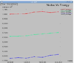
[image:4.595.345.504.611.745.2]

7.1 Simulation Result:

Figure 4: Nodes Vs Energy with multiple sinks

No. of Nodes 200

Area Size 400 m X 200 m

Mac 802.11

Traffic Source CBR

Packet Size 500 bytes

Transmit Power 0.02 mw

Receiving Power 0.01 mw

Idle Power 0.2 mw

Initial Energy 20 J

Figure. 4 shows the relationship between energy consumption and number of sensor nodes that are deployed in the sensing region using MASP with multiple mobile sinks . The curve in red color denotes the energy consumption using single mobile sink.The curve in green color represents the energy consumption using 2 mobile sink.The curve in blue color represents the energy consumption using 3 mobile sink.It clearly shows that the energy consumption is decreased , as the number of mobile sinks increased.

8. CONCLUSION

This paper analyzes the performance of the usage of multiple mobile sinks in collecting the data in wireless sensor networks with reduced energy consumption .The Bi-Stage communication protocol is extended to support multiple mobile sinks and its performance is monitored. This work can be enhanced in future work to focus on addressing the various data storage overheads, and packet delivery ratio.

9. REFERENCES

[1] R.C. Shah, S. Roy, S. Jain, and W. Brunette, “Data MULEs: Modeling a Three-Tier Architecture for Sparse Sensor Networks,” Proc. First IEEE Int’l Workshop Sensor Network Protocols and Applications, pp. 30-41, 2003.

[2] S. Jain, R.C. Shah, W. Brunette, G. Borriello, and S. Roy, “Exploiting Mobility for Energy Efficient Data Collection in Sensor Networks,” Mobile Networks and Applications, vol. 11, no. 3, pp. 327-339, 2006.

[3] A. Chakrabarti, A. Sabharwal, and B. Aazhang, “Communication Power Optimization in a Sensor Network with a Path-Constrained Mobile Observer,” ACM Trans. Sensor Networks, vol. 2, no. 3, pp. 297-324, Aug. 2006.

[4] L. Song and D. Hatzinakos, “Architecture of Wireless Sensor Networks with Mobile Sinks: SparselyDeployed Sensors,” IEEE Trans. Vehicular Technology, vol. 56, no. 4, pp. 1826-1836, July 2007.

[5] Shuai Gao,Hongke Zhang, and Sajal K. Das,”Efficient Data Collection in Wireless Sensor Networks with Path Constrained Mobile Sinks “ IEEE Transactions on Mobile Computing,vol. 10,no.5,pp.592-608,April 2011.

[6] D. Jea, A. Somasundara, and M. Srivastava, “Multiple ControlledMobile Elements (Data Mules) for Data Collection in Sensor Networks,” Proc. First IEEE/ACM Int’l Conf. Distributed Computing in Sensor Systems (DCOSS), pp. 244-257, 2005.

[7] A. Kansal, A. Somasundara, D. Jea, M. Srivastava, and D. Estrin, “Intelligent Fluid Infrastructure for Embedded Networks,” Proc. ACM MobiSys, pp. 111-124, 2004.