www.hydrol-earth-syst-sci.net/16/849/2012/ doi:10.5194/hess-16-849-2012
© Author(s) 2012. CC Attribution 3.0 License.
Earth System
Sciences
Quantifying the contribution of glacier runoff to streamflow in the
upper Columbia River Basin, Canada
G. Jost1,2, R. D. Moore1,2, B. Menounos3, and R. Wheate3
1Department of Geography, Univ. of British Columbia, Canada
2Department of Forest Resources Management, Univ. of British Columbia, Canada
3Natural Resource and Environmental Studies Institute and Geography Program, Univ. of Northern British Columbia, Canada
Correspondence to: R. D. Moore ([email protected])
Received: 30 April 2011 – Published in Hydrol. Earth Syst. Sci. Discuss.: 17 May 2011 Revised: 1 December 2011 – Accepted: 10 December 2011 – Published: 19 March 2012
Abstract. Glacier melt provides important contributions to
streamflow in many mountainous regions. Hydrologic model calibration in glacifed catchments is difficult because er-rors in modelling snow accumulation can be offset by com-pensating errors in glacier melt. This problem is particu-larly severe in catchments with modest glacier cover, where goodness-of-fit statistics such as the Nash-Sutcliffe model ef-ficiency may not be highly sensitive to the streamflow vari-ance associated with glacier melt. While glacier mass bal-ance measurements can be used to aid model calibration, they are absent for most catchments. We introduce the use of glacier volume change determined from repeated glacier mapping in a guided GLUE (generalized likelihood uncer-tainty estimation) procedure to calibrate a hydrologic model. This approach is applied to the Mica basin in the Canadian portion of the Columbia River Basin using the HBV-EC hy-drologic model. Use of glacier volume change in the cali-bration procedure effectively reduced parameter uncertainty and helped to ensure that the model was accurately predict-ing glacier mass balance as well as streamflow. The sea-sonal and interannual variations in glacier melt contributions were assessed by running the calibrated model with historic glacier cover and also after converting all glacierized areas to alpine land cover in the model setup. Sensitivity of modelled streamflow to historic changes in glacier cover and to pro-jected glacier changes for a climate warming scenario was as-sessed by comparing simulations using static glacier cover to simulations that accommodated dynamic changes in glacier area. Although glaciers in the Mica basin only cover 5 % of the watershed, glacier ice melt contributes up to 25 % and 35 % of streamflow in August and September, respectively. The mean annual contribution of ice melt to total streamflow
varied between 3 and 9 % and averaged 6 %. Glacier ice melt is particularly important during warm, dry summers follow-ing winters with low snow accumulation and early snowpack depletion. Although the sensitivity of streamflow to historic glacier area changes is small and within parameter uncertain-ties, our results suggest that glacier area changes have to be accounted for in future projections of late summer stream-flow. Our approach provides an effective and widely appli-cable method to calibrate hydrologic models in glacier fed catchments, as well as to quantify the magnitude and timing of glacier melt contributions to streamflow.
1 Introduction
In many mountainous regions, glacier melt makes signifi-cant contributions to streamflow, particularly in late summer during periods of warm, dry weather (Koboltschnig et al., 2008; Stahl and Moore, 2006; Verbunt et al., 2003; Zappa and Kan, 2007). Understanding the quantity and timing of these contributions is important for a range of purposes, cluding short-term and seasonal forecasting of reservoir in-flows and long-term projections of the potential hydrologic effects of climate change. This knowledge is particularly critical given that these contributions are likely to decrease in the medium to longer term as glaciers retreat (Gurtz et al., 2003; Koboltschnig et al., 2008; Marshall et al., 2011; Stahl et al., 2008), with implications for both water resources man-agement and aquatic ecology (Moore et al., 2009; Zappa and Kan, 2007).
Fig. 1. Location of the Mica basin and locations of climate stations used to force the hydrological model.
glacierized areas”, which by definition also includes the snow melt component, while Stahl et al. (2008) reported only the glacier ice melt component as the relevant contri-bution of glaciers to streamflow because that is the compo-nent that diminishes as a direct result of glacier retreat. In catchments where glacier mass balance and snowline obser-vations exist, a water balance approach can be used to es-timate glacier ice melt contributions to streamflow (Sch¨ar et al., 2004; Young, 1982). Alternatively, empirical analy-sis of the contrasting responses of glacier-fed and unglacier-ized catchments can provide insight (Stahl and Moore, 2006; Schaefli and Huss, 2011). Deterministic hydrologic mod-els can also be used to quantify glacier melt contributions to streamflow (Koboltschnig et al., 2008; Schaefli and Huss, 2011; Stahl et al., 2008). The use of models to quantify glacier melt contributions to streamflow requires adequate representation and parameterization of glacier ice melt pro-cesses. However, in cases where streamflow observations are the only available data for model calibration, an incorrect simulation of glacier ice melt can be offset by compensat-ing errors in the simulation of snow accumulation and snow melt (Konz and Seibert, 2010; Schaefli and Huss, 2011; Stahl et al., 2008), resulting in “equifinality” – i.e. the existence of multiple parameter sets that provide adequate stream-flow simulations despite differences in predictions of snow and ice processes. Equifinality introduces substantial un-certainty into model-based estimates of glacier melt contri-butions to streamflow. Problems associated with equifinal-ity can be reduced by constraining a model with additional information. Previous studies that quantified the contribu-tion of glacier melt to streamflow reduced equifinality by incorporating glacier mass balance data or equilibrium line
altitudes, in addition to streamflow data (Konz and Seibert, 2010; Moore, 1993; Schaefli et al., 2005; Stahl et al., 2008). Unfortunately, glacier mass balance observations are sparse and typically unavailable for most catchments.
Most modelling studies that focused on glacier melt con-tributions to streamflow examined catchments with substan-tial glacier cover, typically in excess of 10 % of the catch-ment area (Koboltschnig et al., 2008; Schaefli and Huss, 2011; Stahl et al., 2008). However, Stahl and Moore (2006) found that the effects of glacier cover on late-summer stream-flow can be detected in catchments with as little as 2 to 5 % glacier coverage. Equifinality may be especially problem-atic in large catchments with modest glacier cover (less than 10 %) given the relatively small variance in streamflow as-sociated with glacier melt contributions. In a recent study focused on macro-scale catchments in Europe with low or modest glacier coverage, Huss (2011) stated that “[m]ass bal-ance data for 50 glaciers in the Swiss Alps . . . [were] cen-tral to this study”. Such extensive glacier mass balance data sets are uncommon outside Europe, limiting the geographic transferability of the approach to other larger catchments out-side Europe.
Another challenge in modelling glacier melt contributions to streamflow is that they can be influenced by changes in glacier cover. In catchments with high glacier cover, sev-eral studies demonstrated that projected glacier changes over the next few decades need to be accounted for in hydrologic modelling to avoid biased predictions (Gurtz et al., 2003; Koboltschnig et al., 2008; Stahl et al., 2008). However, it is not clear from the current literature if accounting for future glacier changes is also necessary in large catchments with modest glacier cover. It is also uncertain how sensitive hy-drologic simulations are to historic changes in glacier cover, particularly over recent decades.
The objective of this study was to develop an approach for estimating the magnitude and timing of glacier melt contribu-tions to streamflow in large catchments with modest glacier cover and no mass balance observations, along with an as-sessment of uncertainty. This study used glacier volume and area changes to assist in calibration, which were derived from analyzing sequential digital elevation models (DEM) and maps of glacier cover. In addition, we address the sen-sitivity of modelled streamflow to historic changes in glacier cover, and to projected glacier changes for a typical climate warming scenario.
2 Methods
2.1 Study area
level (a.s.l.) at Mica dam (MCA in Fig. 1) to 3685 m a.s.l. Based on weather stations in the catchment, mean annual precipitation is 1075 mm, approximately 70 % of which falls as snow. Mean annual temperature is 1.9◦C with monthly av-erage values ranging from−9.4◦C in January to 13.4◦C in July. In 1985, glaciers covered 1268 km2in the Mica basin, representing 6.1 % of the total basin area. Between 1985 and 2000, glacier area decreased by 101 km2, and an addi-tional 80 km2of glacier area was lost between 2000 and 2005 (Bolch et al., 2010), thus reducing glacier cover to 5.2 % of the basin area. About 50 % of the basin consists of open land cover types (i.e. alpine areas, range lands, agricultural lands, recently logged areas), and about 45 % of the area is forested.
2.2 Data
Data from five climate stations within or just outside Mica basin were available for modelling (Fig. 1). Mica dam cli-mate station (MCA) has the longest clicli-mate record, dating back to 1965. Rogers Pass climate station (RGR) data start in 1967, Radium climate station (RAD) in 1969, Molson Creek climate station (MOL) in 1986, and Floe Lake (FLK) climate station in 1993. Backfilled climate data were needed to cal-culate historic changes in streamflow. To extend the records for all climate stations back to 1965, we computed propor-tionality factors for each three-month quarter to rescale pre-cipitation data from MCA, while air temperatures were esti-mated based on linear regressions for each quarter of the year. Only measured climate data were used for model calibration and testing, except for eight years of backfilled data from FLK (1985–1993). Errors associated with air temperature measurements, instrumental error and the possibility of bias associated with site characteristics are believed to be small relative to spatial and temporal variability in Mica basin.
Streamflow data used in this study are daily inflows to Kinbasket Reservoir, computed by BC Hydro from a wa-ter balance based on the rates of release through the dam and changes in water level. Although evaporation from the reservoir is not included in the computed inflows, estimates based on reservoir area and potential evaporation indicate it should not exceed about 1 % of inflow. BC Hydro calcu-lates an estimate of the average daily inflow error as the root mean squared error (RMSE) between quality-controlled and raw inflow data for all their reservoirs (F. Weber, BC Hydro, personal communication, 2011). The RMSE for daily Mica inflow observations is approximately 10 %. For monthly and annual data, where daily random errors are likely to cancel out, RMSE was not calculated but should be smaller than the daily error and primarily reflect the presence of systematic errors.
Snow water equivalent (SWE) data for three snow pil-lows located at the FLK, MOL, and RGR climate stations (Fig. 1) were available from 1995 onwards. Glacier cover-ages were derived from Landsat Thematic Mapper scenes for 2005 and 2000 and from high altitude aerial photography for
1985 (Bolch et al., 2010). Glacier volume loss was calcu-lated from digital elevation models (DEM) derived from the 1999 Shuttle Radar Topography Mission (SRTM) and from aerial photographs taken between 1982 and 1988, which have a median weighted date for Mica basin of 1985 (Schiefer et al., 2007). The estimated ice volume loss from 1985–1999 was 7.75 km3. Taking mapping uncertainty into account, ice volume loss from 1985–1999 lies between 6 and 9 km3.
The geodetic estimate of the rate of thickness change for the Columbia region of British Columbia was−0.53 m yr−1 (Schiefer et al., 2007), while the rate specifically for Mica basin was−0.43 m yr−1. This rate of thinning is slightly less than that indicated by in situ measurements of mass balance at Peyto Glacier, Alberta, which averaged approximately −0.6 m yr−1between 1966 and 2005 (Statistics Canada, last access: 21 October 2011). Peyto Glacier is located to the east of Mica basin in the Rocky Mountains, which receives less snowfall than Mica basin. Therefore, the difference between the rates of mass loss for Mica basin and Peyto Glacier is consistent with the differences in the climatic settings.
2.3 The HBV-EC hydrologic model
The HBV-EC model is a Canadian variant of the HBV-96 model (Lindstrom et al., 1997). It has been incorporated into the EnSim Hydrologic modelling environment (now known as Green Kenue) (Canadian Hydraulics Centre, 2010). The ability of HBV-EC to provide accurate predictions of stream-flow in British Columbia’s mountain catchments was demon-strated in an intercomparison study of watershed models for operational river forecasting (Cunderlik et al., 2010; Fleming et al., 2010). The model algorithms have been described in detail by Hamilton et al. (2000), Canadian Hydraulics Cen-tre (2010) and Stahl et al. (2008). Key features are presented below.
To minimize computational effort, HBV-EC is based on the concept of grouped response units (GRUs), which con-tain grid cells having similar elevation, aspect, slope, and land cover. HBV-EC has the capability to model four land-cover types: open, forest, glacier and water. To represent lateral climate gradients, HBV-EC allows for subdividing a basin into different climate zones, each of which is associ-ated with a single climate station and a unique parameter set. Water draining from non-glacier GRUs is routed through two lumped reservoirs representing “fast” and “slow” responses. To predict the discharge for a given time step, HBV-EC sums output from the two non-glacier reservoirs and the reservoirs associated with glacier GRUs (see below).
The temperature-index-based snow melt algorithm from HBV-96 was adapted by Hamilton et al. (2000) to account for the effects of slope,s, aspect,a, and forest cover. In HBV-EC, daily snowmelt (M) (mm day−1) is calculated from daily mean air temperature (Tair) (◦C) as follows:
whereC0is a base melt factor (mm day−1◦C−1) that varies sinusoidally between a minimum value (Cmin) at the winter solstice to a maximum value at the summer solstice (Cmin+ 1C) to account for seasonal variations in solar radiation, and 1Cis the increase in melt factor between winter and summer solstices. The melt ratio for forests (MRF) ranges between 0 and 1 and reduces melt rates under forests compared to melt at open sites. The coefficient AM controls the sensitivity of melt rates to slope s and aspecta and thus mimics the effects of spatial variations in solar radiation. For glacier GRUs, melt is computed as for an open site (MRF=1) until the previous winter’s snow accumulation has ablated. At that point, glacier melt is computed by multiplying open site melt by the coefficient MRG, which typically ranges between 1 and 2, to represent the reduction in surface albedo.
Storage and drainage of meltwater and rain for each glacier GRU are modelled using linear reservoirs. The out-flow coefficient (KG) for each GRU depends on snow depth, ranging from a low value (KGmin) when the GRU has deep snow cover to a maximum value (KGmin+1KG) when the GRU is snow-free (Stahl et al., 2008). This representation accounts for seasonal changes in the efficiency of the glacier drainage system. Glaciers in HBV-EC cannot vary in area or volume during a model run without stopping and restarting the simulation. The net mass balance for each GRU is calcu-lated from time series of SWE and glacier ice melt for each glacier GRU. The total mass balance for the Mica basin is calculated from area-weighted net mass balances from each elevation band. For more details see Stahl et al. (2008).
2.4 Calibration and testing
The model was calibrated for the period 1985–1999, the same period for which the glacier volume loss was calcu-lated. Calibration runs were split into two time periods, each with a five-year spin-up period to ensure that storages in the model, in particular the slow reservoir storage, equilibrated with the forcing data. Simulations for the first period, 1985– 1992, used the 1985 glacier coverage, while the second pe-riod, 1992–1999, was based on glacier coverage from 2000. The updating of glacier area during the model calibration was done to be consistent with the updating in a long term sim-ulation to assess the importance of glacier area updating de-scribed in Sect. 2.7, below. Glacier net mass balance (bn) for the entire basin was derived from net mass balances for each GRU and compared to geodetically calculated glacier volume loss.
The period 2000–2007, with glacier cover based on data from 2005, was used as an independent test period. Model predictions were compared to observed streamflow data and SWE data from the three snow pillow sites (FLK, MOL, RGR, in Fig. 1). Although HBV-EC does not explicitly represent temporal variability in precipitation and tempera-ture lapse rates, our model setup does account for some de-gree of seasonal variability in vertical climatic gradients by
delineating Mica basin into five climate zones – partly based on elevation – and forcing each climate zone with a sepa-rate climate station. Since HBV-EC does not predict state variables for a specific location but only for each GRU, ob-served SWE data were compared with simulated SWE from the GRUs in which the snow pillows are located. The SWE data were not used in model calibration, and thus represent an independent test of the model.
2.5 A “guided” GLUE approach to address parameter
uncertainty
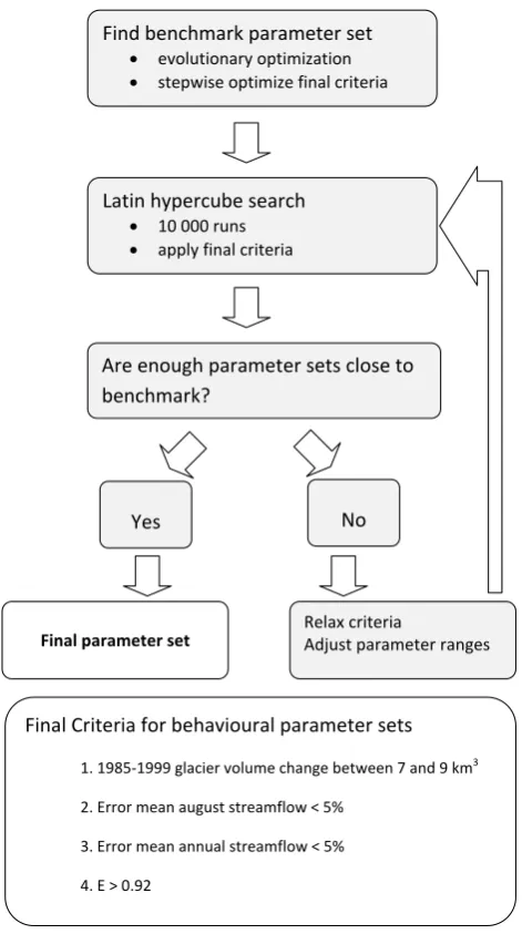
A common approach to address uncertainty in model predic-tions is to generate random samples from the usually high-dimensional parameter space and subsequently to pick the best performing parameter sets according to one or multiple criteria (e.g. Konz and Seibert, 2010; Stahl et al., 2008, for glacier related applications). However, in a high-dimensional parameter space, random sampling with even thousands of model runs does not guarantee that the “best” parameter combinations are found. Without prior knowledge of how well the “best” possible solution performs, the modeller will usually relax criteria in order to obtain enough acceptable parameter sets, with the possible result that criteria for ac-ceptable parameter sets are more relaxed than necessary. Par-ticularly in large catchments with moderate glacier cover, this approach could result in high uncertainties for glacier ice melt estimates. To ensure that the final ensemble parame-ter set contains solutions that perform similarly to the “best” possible solution(s) within a parameter space, we modified the Generalized Likelihood Uncertainty Estimation (GLUE) approach outlined in Beven and Freer (2001) and Freer et al. (1996) to an approach that can be described as a “guided” GLUE approach (Fig. 2).
Find benchmark parameter set
• evolutionary optimization
• stepwise optimize final criteria
Are enough parameter sets close to benchmark?
Latin hypercube search
• 10 000 runs
• apply final criteria
Yes
Relax criteria
Adjust parameter ranges No
Final parameter set
Final Criteria for behavioural parameter sets
1. 1985‐1999 glacier volume change between 7 and 9 km3
2. Error mean august streamflow < 5%
3. Error mean annual streamflow < 5%
[image:5.595.50.286.60.482.2]4. E > 0.92
Fig. 2. Flow chart illustrating the “guided” GLUE approach for cal-ibration and uncertainty analysis.Eis the Nash-Sutcliffe efficiency.
prior parameter distributions (decrease the ranges). Increas-ing the sample size is the favored solution because it should lead to a more diverse set of parameters. However, the num-ber of model runs is limited by computational power (even with multiple CPUs it would take weeks for Mica basin). Given time constraints, we chose to adjust the prior parame-ter distributions. With adjusted (narrowed) parameparame-ter ranges, the LHS was repeated until enough parameter sets (∼20–30) were found that fulfilled all criteria (i.e. “behavioral” para-meter sets in GLUE terminology). The parapara-meter ranges for model calibration and uncertainty analysis were based on de-fault values provided in the HBV-EC manual (Canadian Hy-draulics Centre, 2010), values reported in previous studies (Hamilton et al., 2000; Stahl et al., 2008), the authors’ ex-perience with applying HBV-EC on other catchments, and
by visually testing the influence of parameters on the sim-ulated hydrograph. With the modest glacier cover in Mica, a visual inspection of simulated hydrographs provided more information on the sensitivity of modelled streamflow to the various glacier parameters than a single goodness of fit mea-sure such asE. Prior parameter distributions for LHS were assumed uniform at all stages.
2.6 Assessing the sensitivity of streamflow to glacier
area changes
To assess the sensitivity of streamflow simulations to historic glacier area changes, we compared simulations for the lat-ter part of the test period using the earliest glacier coverage (1985) to contrast with the simulations based on the 2005 coverage (which was used for the latter part of the test pe-riod). We also assessed the sensitivity of simulated stream-flow to projected changes in glacier area under a typical cli-mate warming scenario by comparing ensemble simulations using a static (observed) glacier cover from 2005 throughout the 100 yr simulation period to simulations with a dynamic glacier cover. Forcings for HBV-EC were based on simula-tions from one global climate model (GCM), the Canadian CGCM3.1-T47, with the A1B emissions scenario, which represents a mid-range warming scenario (Nakicenovic et al., 2000). Daily output from the GCM was downscaled for input to HBV-EC using the TreeGen algorithm (Stahl et al., 2008). Projected changes in glacier cover under the A1B emission scenario, also derived from CGCM3.1-T47, were simulated using the UBC Regional Glaciation Model, a physically based, spatially distributed model of glacier dy-namics (G. Clarke, The University of British Columbia, per-sonal communication, 2011; Clarke et al., 2011). At the time of writing, publications describing the Regional Glaciation Model and its application to the Columbia Mountains are in preparation, so we cannot provide details of model out-put here. The objective here was not to present comprehen-sive projections of future changes to inflow, but rather to help identify if and when glacier area updating is of relevance in a large basin with modest glacier cover; hypothetical glacier decreases could have been used as an alternative. Model out-put indicates that glacier area will decrease by 83 % of the glacier extent in 2000 by the end of this century.
2.7 Modelling the contributions of glacier ice melt to
streamflow
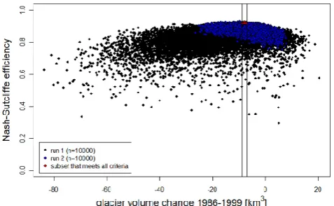
Fig. 3. Nash-Sutcliffe efficiency (E) plotted against simulated glacier volume change for 10 000 model runs in the initial Latin Hypercube Search (black) and for 10 000 model runs in a Latin Hy-percube Search with adjusted prior parameter distributions (blue). Red dots indicate acceptable parameter combinations.
To accommodate changes in the glacier extents and eleva-tions through time, HBV-EC was run using scripts that would update the glacier GRUs used in the simulations based on the observed glacier extents in 1985, 2000, and 2005. The updating involved stopping the simulation, reading in the new glacier extents, updating the definitions of Grouped Re-sponse Units and state variables, and then continuing the sim-ulation, including a five year spin-up period. Transient runs from 1972 to 2007 were obtained by running HBV-EC from 1972 to 1992 with the observed 1985 glacier cover, from 1993 to 2000 with the glacier cover from 2000, and from 2001 to 2007 with the observed 2005 glacier cover. The as-sumption that glacier areas did not change appreciably from 1972 to 1985 is supported by physically based distributed modelling of glacier dynamics (G. Clarke, The University of British Columbia, personal communication, 2011). Transient future simulations were obtained by updating the glacier area in 10 yr intervals from 1970 to 2100, again with five year spin-up periods before running the model for 10 yr. The his-torical period 1970 to 2000 serves as a baseline.
3 Results
3.1 Model calibration and uncertainty analysis
[image:6.595.310.549.61.216.2]The benchmark parameter set obtained by the combined evolutionary-steepest gradient optimization matched ob-served streamflow data withEof 0.93 for the calibration pe-riod (1985–1999) and 0.95 for the test pepe-riod (2000–2007). A first 10 000 run LHS within the initial parameter ranges (parameter range step 1 in Fig. 2) found no acceptable para-meter sets that met all criteria. Although 28 parapara-meter sets hadE >0.91, all of these parameter sets were rejected be-cause none fulfilled all of the additional criteria. In the
Fig. 4. Observed and simulated discharge for the test period (2000– 2007). (a) observed and simulated discharge predicted with the best performing (E) parameter set; (b) observed and the ensemble of simulated discharge.
absence of prior knowledge of the benchmarkE, the com-mon procedure would now have been to find acceptable so-lutions with relaxed criteria. However, the benchmark para-meter set indicates that there are better performing solutions within the initial parameter space; 10 000 runs are too few to sample the parameter space for acceptable solutions. A sec-ond LHS with adjusted parameter ranges found 17 acceptable parameter sets, but histograms indicated that two parameters in the acceptable parameter sets were predominantly sam-pled near a range boundary and therefore a third LHS with slightly refined parameter ranges was performed. From the 10 000 model runs in the third LHS, 705 parameter sets met the final criterion ofE >0.92, but only 23 of these also met the additional criteria (Fig. 2).
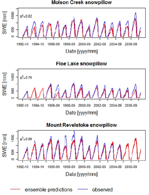
Fig. 5. Ensemble simulated and observed snow water equivalents for three snow pillow sites. Simulations are for the GRU that cor-responded to the snow pillow sites, and show the 5–95 % quantile range.
A wide range of modelled glacier volume changes can lead to values of E close to the benchmark (Fig. 3). Re-sults from the first LHS suggest that equifinal parameter so-lutions are possible with glacier volume losses ranging from 5 to 40 km3. This point underlines the advantage of using observed glacier volume changes to constrain model param-eters, particularly in large basins with modest glacier cov-erage like Mica. Note that the second LHS gives higher maximum values ofEbecause of the greater sampling den-sity within the restricted parameter space and not necessar-ily because the glacier volume loss is close to the observed. More intense sampling within the parameter space that leads to higher glacier volume losses could possibly have led to higherEat higher glacier volume losses as well. Combina-tions that lead to increases in glacier volume yielded a sub-stantial decrease inE.
3.2 Model testing
Model testing on streamflow for the period 2000–2007, us-ing the observed glacier extents from 2005, yielded an effi-ciency of 0.95 for the best model (Fig. 4a), a slightly better
Fig. 6. The effect of glaciers on mean annual discharge shown by comparing simulations with and without glaciers including uncer-tainty limits (5–95 % quantile range).
performance than during the 1985–1999 calibration period (E=0.93). The goodness of fit of the best parameter set de-rived by the Latin hypercube search is essentially the same as the fit obtained by the combined evolutionary-steepest gradi-ent optimization.
All 23 behavioral parameter sets reproduce the seasonal peak flows as well as low flows, but have difficulty with modelling intense rainfall events, especially during autumn (Fig. 4b). This is not surprising, since one of the two reser-voirs (the slow reservoir) is primarily used to model the low flows during winter, and the single fast reservoir cannot si-multaneously represent runoff generation due to melt and rainfall given the differences in their spatial patterns and non-linearity. Since this model weakness only appears to affect rainfall-generated daily peak flows, it should not detract from the estimation of glacier melt contributions to streamflow, es-pecially over monthly or longer time scales.
[image:8.595.46.290.63.381.2]Fig. 7. The effect of glaciers on mean August discharge shown by comparing simulations with and without glaciers including uncer-tainty limits (5–95 % quantile range).
Fig. 8. The effect of glaciers on mean September discharge shown by comparing simulations with and without glaciers including un-certainty limits (5–95 % quantile range).
Lake. Inconsistent variations in gauge catch efficiency could explain at least some of this underprediction. This incon-sistent pattern of errors could also partly reflect the inherent variability in precipitation patterns from year to year, which are probably not fully represented through the use of fixed vertical gradients in each climate zone.
3.3 Historic contributions of glacier ice melt to
streamflow
The mean annual contribution of ice melt to total streamflow varied between 3 and 9 % and averaged 6 % (Fig. 6). Trend analysis revealed no significant increase or decrease of the annual contributions of glacier ice melt with time. For an-nual, August and September flows, the uncertainty bounds between runs with and without glaciers are close but do not overlap for most years (Figs. 6 to 8).
Contributions of glacier ice melt to discharge at Mica dam dominantly occur in August and September (Figs. 7 and 8). Mean August streamflow, calculated from the en-semble mean, would be up to 25 % lower if there were no
Fig. 9. The effect of glaciers on discharge shown by comparing simulations with and without glaciers for the year with the high-est modelled ice melt (1998) and the year with the lowhigh-est ice melt (2000).
glaciers, although the interannual variation of contributions is relatively high (standard deviation = 7 % of the simulated mean flow with glaciers) (Fig. 7). The relative contribution of glaciers is highest in September, when ice melt can pro-vide up to 35 % of the discharge. September contributions of ice melt are also less variable over time, with a standard deviation of 5 % of the simulated mean flow with glaciers (Fig. 8).
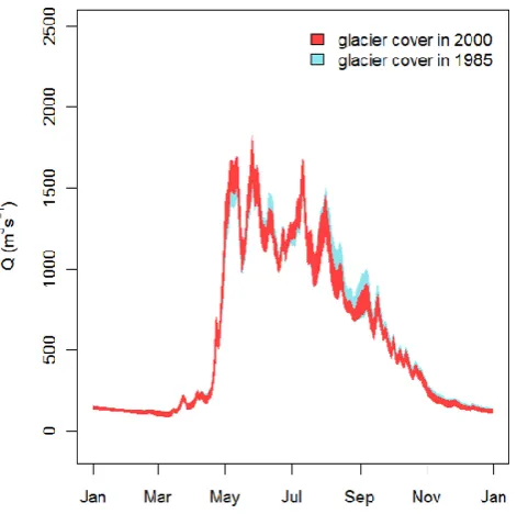
[image:9.595.50.285.260.396.2]Fig. 10. Illustration of the sensitivity of simulated streamflow to glacier changes during the calibration period, based on a compar-ison of ensemble simulations for the year 1998 using the glacier coverages from 1985 and 2000.
3.4 Sensitivity of streamflow to glacier area changes
Figure 10 presents the sensitivity of streamflow to histori-cal glacier area changes by comparing streamflow simula-tions using the earliest glacier coverage (1985) with the sim-ulations based on the 2000 glacier coverage for 1998, the year with the highest historical glacier icemelt. Although late summer flows are lower for simulations based on the smaller glacier coverage in 2000, the sensitivity of streamflow to his-torical glacier area changes is small and within the variation associated with parameter uncertainty.
Averaged over the Mica basin, the climate scenario based on the A1B emission scenario generates a warming of 3.0◦C and an 11 % increase in precipitation. Figure 11 shows that the effect of glacier retreat on predicted streamflow can be significant, depending on the stage and rate of deglaciation. Differences between the simulations for static and dynamic glacier cover start to emerge from parameter uncertainty around 2060, when glacier area decreased by 40 % relative to the glacier area in 2000.
4 Discussion
The Nash-Sutcliffe efficiencyEexhibits an optimum value associated with negative glacier volume change; i.e. para-meter sets that incorrectly predict positive mass balance do a worse job of predicting streamflow. In contrast to other studies (e.g. Stahl et al., 2008), the optimal value ofEcan
Fig. 11. Ensemble simulations of mean August streamflow for a climate scenario based on the A1B emissions scenario using a static glacier cover (based on the observed glacier cover in 2005) and a dynamic glacier cover.
be achieved by a wider range of glacier volume changes (−5 to−40 km3), which reflects the modest glacier cover in the large Mica basin and the associated lower sensitivity of streamflow to glacier melt, relative to studies of more heav-ily glacierized catchments. However, even if there had been a narrow peak ofEover glacier volume loss (like in Stahl et al., 2008), Schaefli and Huss (2011) showed that one has to be careful not to infer glacier volume loss from such a relation since, due to potential model structural errors, the “real” glacier volume loss does not need to coincide with the glacier volume loss that gives the best model performance. Because Stahl et al. (2008) had winter mass balance mea-surements, they were able to fix the climate parameters,Tlapse andPlapse, at an initial step during model calibration, sepa-rately from the calibration using streamflow data. In con-trast, our approach does not allow climate related parameters to be calibrated independently from the streamflow simula-tions. Hence, a greater amount of uncertainty in these param-eters (wider parameter ranges) is propagated through to our streamflow predictions.
[image:10.595.309.547.60.255.2]that even glacier-wide volume change spanning several years can constrain model parameters such that the glacier ice con-tribution to streamflow can be quantified with reduced un-certainty. Given the general lack of mass balance data world-wide, our approach should prove useful for assisting in model calibration, particularly in large basins with modest glacier cover, where goodness-of-fit indices like the model effi-ciency are less sensitive to the streamflow variability related to glacier contributions. If a hydrologic model will be used to make future projections of the effects of climate change, it is imperative that a model be able to simulate glacier mass balance with reasonable accuracy, not just streamflow.
Given that repeated DEM mapping may only be avail-able over periods of a decade or more, the approach applied here will require relatively long calibration periods – 15 yr in the case of Mica basin. The future projections (Fig. 11) demonstrate that changes in glacier area over decadal time scales can potentially have a significant influence on summer streamflow. Therefore, under conditions of rapid glacier re-treat, it may be necessary to represent the effects of glacier shrinkage during the calibration period, even in large catch-ments like Mica basin with modest glacier cover. Current long term planning data sets for the Columbia Region, used for example in hydroelectric operations planning, either do not account for glaciers (Hamlet et al., 2010) or assume static glaciers (Schnorbus et al., 2011; B¨urger et al., 2011). Our results suggest that, for climate change impact assess-ments where glaciers are projected to recede substantially, the effects of glacier recession on streamflow have to be con-sidered even in basins with modest glacier cover (less than 10 %).
It is awkward to incorporate automated glacier area up-dates during model calibration and during long-term future projections using a model like HBV-EC, which represents a basin using static land cover. In our study, these updates were accomplished using rather complicated scripting. Despite the efficient structure of HBV-EC, which employs grouped re-sponse units and lumped reservoirs, the calibration process took substantial processing time (one week for 10 000 model runs on five CPUs, two weeks for the evolutionary optimiza-tion on one CPU). This challenge is not unique to the HBV-EC model, since most existing model codes that we are aware of do not allow for changes in land cover during a simulation run. One solution would be to develop a new model code that can accept updated land cover information without having to stop and restart execution.
Glacier contributions to Mica basin streamflow are great-est in August and September. Although minor in terms of long-term average flows, glacier ice melt is especially impor-tant during relatively warm, dry weather in summers follow-ing a winter with low snow accumulation and early snowpack depletion. These conditions can be critical from both water supply and ecological perspectives. Therefore, water man-agers and aquatic ecologists need to appreciate the hydro-logic significance of glacier melt, even in large basins with
moderate glacier cover. In a large basin such as Mica, glacier ice melt can contribute up to 25 % to 35 % of late summer streamflow.
5 Conclusions
Use of glacier volume change in the calibration procedure ef-fectively reduced parameter uncertainty and helped to ensure that the model was accurately predicting glacier mass bal-ance as well as streamflow. This approach should be widely useful for quantifying glacier contributions to streamflow in glacier-fed catchments where mass balance observations are lacking. One drawback to the approach is that the calibration period must span the interval between glacier maps, in this case 15 yr. Because glacier cover can change significantly over decadal and longer time periods – historically and in future projections – approaches should be developed to ac-commodate glacier cover changes during model simulations. Although glaciers only cover 5 % of the Mica basin, they contributed up to 25 % of mean August flow and 35 % of mean September flow in the historic period. These contri-butions are particularly important during periods of warm, dry weather following winters with low accumulation and early snowpack depletion. Glacier retreat over the twenty-first century could therefore have significant implications for streamflow during critical late-summer periods.
Acknowledgements. This work was supported financially by
the Canadian Foundation for Climate and Atmospheric Science through its support of the Western Canadian Crysopheric Network, a contract from BC Hydro Generation Resource Management, and a Natural Sciences and Engineering Council of Canada Discovery Grant to RDM. Tobias Bolch and Erik Schiefer contributed to the development of historic glacier masks and digital elevation models. Sean Fleming, Frank Weber and Scott Weston of BC Hydro Generation Resource Management assisted with access to data and project administration. Sean Fleming and Frank Weber also provided detailed reviews of earlier versions of this work. Garry Clarke, Faron Anslow, Alex Jarosch and Valentina Radic conducted the simulations of future glacier response under climatic warming scenarios. Alex Cannon assisted with downscaling GCM output. The anonymous reviewers provided constructive comments that helped us improve the ms.
Edited by: G. Bl¨oschl
References
Beven, K. and Freer, J.: Equifinality, data assimilation, and uncer-tainty estimation in mechanistic modelling of complex environ-mental systems using the glue methodology, J. Hydrol., 249, 11– 29, 2001.
B¨urger, G., Schulla, J., and Werner, A. T.: Estimates of future flow, including extremes, of the Columbia River headwaters, Water Resour. Res., 47, W10520, doi:10.1029/2010WR009716, 2011. Canadian Hydraulics Centre: Green Kenue Reference Manual,
Na-tional Research Council, Ottawa, Ontario, 340 pp., 2010. Clarke, G. K. C., Anslow, F. S., Jarosch, A. H., and Radic, V.:
Pro-jections of the climate-forced deglaciation of western Canada us-ing a regional glaciation model. Presented at the 2011 Fall Meet-ing of the American Geophysical Union, San Francisco, 5–9 De-cember 2011.
Cunderlik, J., McBean, E., Day, G., Thiemann, M., Kouwen, N., Jenkinson, W., Quick, M., and Lence, B. L. Y.: Intercomparison study of process-oriented watershed models, BC Hydro, Rich-mond, BC, 2010.
Fleming, S., Cunderlik, J., Jenkinson, W., Thiemann, M., and Lence, B.: A “horse race” intercomparison of process-oriented watershed models for operational river forecasting, CWRA An-nual Conference, Vancouver, BC, 2010.
Freer, J., Beven, K., and Ambroise, B.: Bayesian estimation of un-certainty in runoff prediction and the value of data: An applica-tion of the glue approach, Water Resour. Res., 32, 2161–2173, 1996.
Gray, D. M. and Male, D. H.: Handbook of Snow: Principles, Pro-cesses, Management and Use, Pergamon Press, New York, 776 pp., 1981.
Gurtz, J., Zappa, M., Jasper, K., Lang, H., Verbunt, M., Badoux, A., and Vitvar, T.: A comparative study in modelling runoff and its components in two mountainous catchments, Hydrol. Processes, 17, 297–311, doi:10.1002/hyp.1125, 2003.
Hamilton, A. S., Hutchinson, D. G., and Moore, R. D.: Estimating winter streamflow using conceptual streamflow model, J. Cold Regions Engineering, 14, 158–175, 2000.
Hamlet, A. F., Carrasco, P., Deems, J., Elsner, M. M., Kamstra, T., Lee, C., Lee, S.-Y., Mauger, G., Salathe, E. P., Tohver, I., and Whitely Binder, L.: Final project report for the Columbia basin climate change scenarios project, available at: http://www. Hydro.Washington.Edu/2860/report/, 2010.
Huss, M.: Present and future contribution of glacier storage change to runoff from macroscale drainage basins in Europe, Water Re-sour. Res., 47, W07511, doi:10.1029/2010wr010299, 2011. Koboltschnig, G. R., Sch¨oner, W., Zappa, M., Kroisleitner, C., and
Holzmann, H.: Runoff modelling of the glacierized alpine upper Salzach basin (Austria): Multi-criteria result validation, Hydrol. Processes, 22, 3950–3964, doi:10.1002/hyp.7112, 2008. Konz, M. and Seibert, J.: On the value of glacier mass balances for
hydrological model calibration, J. Hydrol., 385, 238–246, 2010. Lindstrom, G., Johansson, B., Persson, M., Gardelin, M., and Bergstrom, S.: Development and test of the distributed hbv-96 hydrological model, J. Hydrol., 201, 272–288, 1997.
Marshall, S., White, E., Demuth, M., Bolch, T., Wheate, R., Me-nounos, B., Beedle, M., and Shea, J.: Glacier water resources on the eastern slopes of the Canadian Rocky Mountains, Can. Water Resour. J., 36, 109–134, 2011.
Mebane, W. R. and Sekhon, J. S.: Genetic optimization using derivatives: The rgenoud package for R, J. Stat. Softw., 42, 1– 26, available at: http://www.jstatsoft.org/v42/i11/, 2011. Moore, R. D.: Application of a conceptual streamflow model
in a glacierized drainage basin, J. Hydrol., 150, 151–168, doi:10.1016/0022-1694(93)90159-7, 1993.
Moore, R. D., Fleming, S. W., Menounos, B., Wheate, R., Fountain, A., Stahl, K., Holm, K., and Jakob, M.: Glacier change in west-ern north america: Influences on hydrology, geomorphic hazards and water quality, Hydrol. Processes, 23, 42–61, 2009.
Nakicenovic, N., Alcamo, J., Davis, G., de Vries, B., Fenhann, J., Gaffin, S., Gregory, K., Grubler, A., Jung, T. Y., and Kram, T.: Special report on emissions scenarios: A special report of work-ing group iii of the intergovernmental panel on climate change, Pacific Northwest National Laboratory, Richland, WA (US), En-vironmental Molecular Sciences Laboratory (US), 2000. R Development Core Team: R: A Language and Environment for
Statistical Computing, R Foundation for Statistical Computing, ISBN 3-900051-07-0, available at: http://www.R-project.org, 2011.
Schaefli, B. and Huss, M.: Integrating point glacier mass bal-ance observations into hydrologic model identification, Hy-drol. Earth Syst. Sci., 15, 1227–1241, doi:10.5194/hess-15-1227-2011, 2011.
Schaefli, B., Hingray, B., Niggli, M., and Musy, A.: A con-ceptual glacio-hydrological model for high mountainous catch-ments, Hydrol. Earth Syst. Sci., 9, 95–109, doi:10.5194/hess-9-95-2005, 2005.
Sch¨ar, C., Vidale, P. L., L¨uthi, D., Frei, C., H¨aberli, C., Liniger, M. A., and Appenzeller, C.: The role of increasing temperature variability in European summer heatwaves, Nature, 427, 332– 336, 2004.
Schiefer, E., Menounos, B., and Wheate, R.: Recent volume loss of british columbian glaciers, canada, Geophys. Res. Lett., 34, 1–6, 2007.
Schnorbus, M. A., Bennett, K. E., Werner, A. T., and Berland, A. J.: Hydrologic impacts of climate change in the Peace, Camp-bell and Columbia watersheds, British Columbia, Canada. Pa-cific Climate Impacts Consortium, Victoria, BC, 157, 2011. Stahl, K. and Moore, R.: Influence of watershed glacier coverage on
summer streamflow in British Columbia, Canada, Water Resour. Res., 42, W02422, doi:10.1029/2007WR005956, 2006. Stahl, K., Moore, R. D., Shea, J. M., Hutchinson, D., and Cannon,
A. J.: Coupled modelling of glacier and streamflow response to future climate scenarios, Water Resour. Res., 44, W06201, doi:10.1029/2006WR005022, 2008.
Statistics Canada: Cumulative net mass balance, western cordillera glaciers, available at: http://www.statcan.gc.ca/pub/16-002-x/ 2010003/ct006-eng.htm, last access: 21 October 2011.
Stenborg, T.: Delay of runoff from a glacier basin, Geogr. Ann. A., 52, 1–30, 1970.
Verbunt, M., Gurtz, J., Jasper, K., Lang, H., Warmerdam, P., and Zappa, M.: The hydrological role of snow and glaciers in alpine river basins and their distributed modeling, J. Hydrol., 282, 36– 55, 2003.
Young, G. J.: Hydrological relationships in a glacierized mountain basin, in: Hydrological Aspects of Alpine and High-Mountain Areas, Proceedings of the Exeter Symposium, IAHS Publ. 138, 51–59, 1982.