www.hydrol-earth-syst-sci.net/20/3745/2016/ doi:10.5194/hess-20-3745-2016
© Author(s) 2016. CC Attribution 3.0 License.
Disentangling timing and amplitude errors
in streamflow simulations
Simon Paul Seibert, Uwe Ehret, and Erwin Zehe
Chair of Hydrology, Institute for Water and River Basin Management, Karlsruhe Institute of Technology (KIT), Kaiserstrasse 12, 76131 Karlsruhe, Germany
Correspondence to:Uwe Ehret ([email protected])
Received: 24 March 2016 – Published in Hydrol. Earth Syst. Sci. Discuss.: 30 March 2016 Revised: 13 July 2016 – Accepted: 16 July 2016 – Published: 12 September 2016
Abstract.This article introduces an improvement in the Se-ries Distance (SD) approach for the improved discrimina-tion and visualizadiscrimina-tion of timing and magnitude uncertainties in streamflow simulations. SD emulates visual hydrograph comparison by distinguishing periods of low flow and pe-riods of rise and recession in hydrological events. Within these periods, it determines the distance of two hydrographs not between points of equal time but between points that are hydrologically similar. The improvement comprises an auto-mated procedure to emulate visual pattern matching, i.e. the determination of an optimal level of generalization when comparing two hydrographs, a scaled error model which is better applicable across large discharge ranges than its non-scaled counterpart, and “error dressing”, a concept to con-struct uncertainty ranges around deterministic simulations or forecasts. Error dressing includes an approach to sample em-pirical error distributions by increasing variance contribu-tion, which can be extended from standard one-dimensional distributions to the two-dimensional distributions of com-bined time and magnitude errors provided by SD.
In a case study we apply both the SD concept and a bench-mark model (BM) based on standard magnitude errors to a 6-year time series of observations and simulations from a small alpine catchment. Time–magnitude error characteris-tics for low flow and rising and falling limbs of events were substantially different. Their separate treatment within SD therefore preserves useful information which can be used for differentiated model diagnostics, and which is not contained in standard criteria like the Nash–Sutcliffe efficiency. Con-struction of uncertainty ranges based on the magnitude of er-rors of the BM approach and the combined time and magni-tude errors of the SD approach revealed that the BM-derived
ranges were visually narrower and statistically superior to the SD ranges. This suggests that the combined use of time and magnitude errors to construct uncertainty envelopes implies a trade-off between the added value of explicitly considering timing errors and the associated, inevitable time-spreading effect which inflates the related uncertainty ranges. Which effect dominates depends on the characteristics of timing er-rors in the hydrographs at hand. Our findings confirm that Series Distance is an elaborated concept for the comparison of simulated and observed streamflow time series which can be used for detailed hydrological analysis and model diag-nostics and to inform us about uncertainties related to hydro-logical predictions.
1 Introduction
Manifold epistemic and aleatory uncertainties make the sim-ulation of streamflow a fairly uncertain task. The assessment of uncertainties, i.e. quantification, evaluation, and commu-nication, is thus of great concern in decision making, model evaluation, the design of technical structures like flood pro-tection dams or weirs, and many other issues. The quantifi-cation and evaluation of uncertainties typically involves the comparison of simulated and observed rainfall–runoff data.
from the human ability to identify and compare matching, i.e. hydrologically similar parts of hydrographs (“to compare apples with apples”) and particularly to discriminate verti-cal (magnitude) and horizontal (timing) agreement of hydro-graphs. Whereas the former implies that rising and falling limbs of the two time series are intuitively and meaningfully matched before they are compared, the latter refers to a joint but yet individual consideration of timing and magnitude er-rors. Visual hydrograph inspection is hence a powerful yet demanding evaluation technique which is still rather difficult to mimic by automated methods. Clear disadvantages of vi-sual hydrograph inspection, however, are its subjectivity and that its application is restricted to a limited number of events. 1.1 Single and multiple criteria for hydrograph
evaluation
To overcome this shortcoming, a large number of numeri-cal criteria (Nash and Sutcliffe, 1970; Legates and McCabe, 1999; Pachepsky et al., 2006; Dawson et al., 2007; Laio and Tamea, 2007; Bennett et al., 2013) have been proposed. How-ever, each criterion typically evaluates only one or just a few hydrograph aspects and there is no “one size fits all” solu-tion available. For this reason different attempts have been undertaken to compare expert judgement and automated cri-teria (Crochemore et al., 2014) and to establish model eval-uation guidelines (e.g. Moriasi et al., 2007; Biondi et al., 2012; Harmel et al., 2014). Key points of related guidelines typically include the statement that the choice of the met-ric should depend (i) on the modelling purpose, (ii) on the modelling mode (calibration, validation, simulation, or fore-cast), and (iii) on the model resolution (time stepping, spatial resolution). Further, most authors recommend the combina-tion of several, preferably orthogonal criteria, which might imply combined application of absolute and relative crite-ria (Willmott, 1981). Hence, within the last decade several multi-criteria approaches for model calibration and evalua-tion have been proposed (Gupta et al., 1998; Boyle et al., 2000; Vrugt et al., 2003; Efstratiadis and Koutsoyiannis, 2010; Kollat et al., 2012), which combine different perfor-mance criteria and/or evaluation against hydrological signa-tures such as the shape of the flow duration curve (Euser et al., 2013; Hrachowitz et al., 2014). Even approaches aim-ing to mimic visual hydrograph comparison were developed. These include multicomponent mapping (Pappenberger and Beven, 2004), self-organizing maps (Reusser et al., 2009), wavelets (Liu et al., 2011), the hydrograph matching algo-rithm (Ewen, 2011), and the “Peak-Box” approach for the interpretation and verification of operational ensemble peak-flow forecasts (Zappa et al., 2013). Despite this considerable progress, many practical and scientific applications (Haag et al., 2005; Gassmann et al., 2013; Seibert et al., 2014; Wrede et al., 2014; Kelleher et al., 2015; Zhang et al., 2016) still rely on simple mean squared error (MSE) type dis-tance metrics such as the long-established Nash–Sutcliffe
ef-ficiency (NASH) or the root mean squared error (RMSE) even though their shortcomings are well known (Seibert, 2001; Schaefli and Gupta, 2007; Gupta et al., 2009).
A less recognized issue of MSE-type criteria is that these compare points with identical abscissa, i.e. at the same po-sition in time. This means that points in the observation are “vertically” compared to points in the simulation (in the fol-lowing we refer to them as vertical metrics). The problem with this is that small errors in timing may be expressed as large errors in magnitude. It is obvious that neither individ-ual criteria nor the combination of different vertical metrics within a multi-objective approach can compensate for this. 1.2 Uncertainty assessment and model diagnostics –
learning from model deficiencies
Just as with performance criteria, many methods related to the quantification, visualization, and communication of un-certainties were developed in recent decades, and the value of knowledge about simulation uncertainty is now gen-erally acknowledged. The range of methods is large and comprises manifold probabilistic and non-probabilistic ap-proaches. Probabilistic concepts, for instance, include the to-tal model uncertainty concept (Montanari and Grossi, 2008), methods based on Bayes’ theorem (Krzysztofowicz, 1999; Krzysztofowicz and Kelly, 2000), and various ensemble techniques (Roulston and Smith, 2003; Georgakakos et al., 2004; Cloke and Pappenberger, 2008). Non-probabilistic methods include the generalized likelihood uncertainty es-timation (GLUE) (Beven and Binley, 1992), possibilistic methods (Jacquin and Shamseldin, 2007), or approaches ap-plying fuzzy-set theory (Nasseri et al., 2014). Uncertainty assessment is a field of ongoing research, and so far there is no generally accepted technique available. The most im-portant points of criticism of the non-probabilistic methods are their subjectivity and their inconsistency with probabilis-tic approaches when these are applied to cases which can be explicitly answered using statistical approaches (Stedinger et al., 2008). On the other hand, probabilistic approaches always rely on the assumptions of ergodicity and stationar-ity, which are rarely fulfilled in reality. A spin-off of uncer-tainty assessment is the field of model diagnostics, which ul-timately aims to learn more about and from model deficien-cies. Related approaches either analyse the temporal patterns of parameter identifiability (Wagener et al., 2003) or the coin-cidence of typical errors (Reusser et al., 2009) and parameter sensitivity (Reusser and Zehe, 2011) in streamflow simula-tion.
between the observed and simulated hydrographs are deter-mined for matching pairs of points in the event, but the two distances are kept separate. Such separate treatment is for instance desirable in flood forecasting, where errors in mag-nitude are relevant for dike defence, whereas errors in timing are crucial for reservoir operation. The separation of timing and magnitude errors is further helpful for improving model diagnostics as they point towards different deficiencies in the model structure.
Here we present substantial improvements (Sect. 2) to the original approach of Ehret and Zehe (2011), particu-larly the coarse-graining procedure. We furthermore intro-duce a heuristic approach to visualize timing and magni-tude uncertainties in streamflow simulations by construct-ing two-dimensional uncertainty ranges in Sect. 3. Related to that, we provide and test several quality criteria to eval-uate deterministic uncertainty ranges. The skill of uncer-tainty ranges is still rarely evaluated in hydrology (Franz and Hogue, 2011), and most of the available methods such as rank probability scores (Duan et al., 2007), rank his-tograms, or the usage of different moments of the proba-bility density function (De Lannoy et al., 2006) were de-veloped in climatology (Gneiting et al., 2008; Franz and Hogue, 2011). These approaches typically quantify ensem-ble spread and thus are probabilistic approaches to evalu-ate uncertainty estimation. To our knowledge only few de-terministic approaches, e.g. categorical statistics such as the Brier score or contingency tables or combinations of deter-ministic and probabilistic approaches (Shrestha et al., 2009), are available. In Sect. 4 we test the feasibility of the ad-vanced SD approach in a case study and compare it to a standard benchmark error model. Section 5 contains the re-sults and discussion, Sect. 6 the related conclusions. To fos-ter the use of the SD approach, we publish the SD (Mat-lab) code, licensed under Creative Commons license BY-NC-SA 4.0, together with a ready-to-use sample data set along-side this manuscript. It is accessible via a GitHub reposi-tory https://github.com/KIT-HYD/SeriesDistance (Ehret and Seibert, 2016).
2 Series distance – concept and modifications
SD was developed to resemble the strengths of visual hydro-graph inspection in an automated procedure, which typically rests on the following premises (Ehret and Zehe, 2011):
– Hydrographs contain individual events separated by pe-riods of low flow.
– Events are composed of rising and falling limbs or seg-ments which are separated by peaks and troughs. – These different parts of event hydrographs reflect
differ-ent hydrometeorological processes and should be com-pared individually, so as to not compare apples with or-anges. This is of particular importance if the simulated
0 20 40 60 80 100 120
time (h)
60 80 100 120 140 160 180
d
is
c
h
a
rg
e
(
m
3 s
-1
)
[image:3.612.310.546.70.208.2]observation simulation no-event limit
Figure 1.Time series of observed (black) and simulated (grey)
dis-charge during a hydrological event. The horizontal line represents a user-specific threshold which differentiates between event and non-event periods. The light grey lines represent the Series Distance con-nectors linking hydrologically comparable points in the two time series. Time and magnitude distances are calculated between these points. The black rectangle highlights time steps where a part of the recession of the simulation overlaps with a rising part of the obser-vation (figure from Ehret and Zehe, 2011).
(sim in the following) and observed (obs in the follow-ing) hydrographs do belong to different parts of the hy-drograph at the same time stept(compare black rectan-gle in Fig. 1).
– A comprehensive evaluation of the agreement of match-ing rismatch-ing and fallmatch-ing limbs of two hydrographs requires consideration of both errors in timing and magnitude as this better informs us about ways to improve the model. A simulated rising limb can, for example, match per-fectly with its observed counterpart with respect to val-ues but occur systematically too early or too late, which would indicate the need to adjust model parameters re-lated to runoff concentration and flood routing or to im-prove the related model components.
– A comprehensive comparison of sim and obs should also provide information on the overall agreement with respect to the occurrence of relevant events and times of low flow. This is typically expressed by contingency tables, which contain information about correctly pre-dicted, missed, and falsely predicted events.
These criteria listed above inform about different error sources, and their individual evaluation therefore provides useful information for a targeted model improvement. As SD accounts for all of these aspects, it is not a single formula but rather a procedure which includes the following steps. For each step, the main innovations are described in detail in the sections below.
– Identification and pairing of events (Sect. 2.2). New: routines to read user-specified events and to treat the entire time series as a single, long event.
– Identification, matching, and coarse-graining of seg-ments (Sect. 2.3): New: this part has been completely reworked and now applies the coarse-graining proce-dure.
– Calculation of the distance between matching segments with respect to both timing and magnitude (Sect. 2.4). This is the core of SD, and it is important to note that the distances are computed between points of the hy-drographs considered to be hydrologically similar. New: routines to calculate a scaled magnitude error.
– Calculation of a contingency table which counts match-ing, missmatch-ing, and false events. No changes.
2.1 Hydrograph preprocessing
The application of SD usually requires some preprocess-ing to assure gap-free and non-negative time series of equal length; related routines are now included in the SD code. Further routines are available for the adjustment of con-secutive identical values; the identification of rising and falling limbs requires non-zero gradients and for time se-ries smoothing, which is often necessary due to the pres-ence of sensor-related non-relevant microsegments. Smooth-ing is based on the Douglas–Peucker algorithm (Douglas and Peucker, 1973), which preserves extremes but filters the noise (Ehret, 2016). Preprocessing also involves the identifi-cation of segments, i.e. contiguous periods of rise or fall in the hydrograph. This is based on the slope of the hydrograph computed between two successive time steps.
2.2 Identification and pairing of events
For many aspects of hydrology such as flood forecasting or studies of rainfall–runoff transformation, it is useful to con-sider a hydrograph as a succession of distinct events, usu-ally triggered by rainfall events, separated by periods of low flow. As SD is based on the concept of comparing similar parts of obs and sim hydrographs, it ideally also involves the steps of identifying events both in the obs and sim time ries and then relating the resulting events between the se-ries. On this level, the general agreement of the two series is evaluated with a contingency table, which counts the num-ber of hits (observed events that have a matching simulated counterpart), misses (observed events without a simulated counterpart), and false alarms (simulated events without an observed counterpart). This is also the basis for the further steps of the SD procedure: only for matching pairs of obs– sim events can matching segments of rise and fall within the events be identified and the combined time–magnitude error be computed. For misses, false alarms, and periods of low
flow this is not possible. For these cases, the best indicator of hydrological similarity in obs and sim is similarity in time; i.e. the distance between the observed and simulated hydro-graph can be computed with a standard vertical distance mea-sure. The detection of events in hydrographs and their subse-quent pairing, however, is not trivial and has to our knowl-edge not yet been solved in an automated and generalized way. The original version of SD applied a simple no-event threshold (see Fig. 1) which, however, often produced un-satisfactory results in the form of many non-intuitive misses or false alarms if the events peaked just above or below the threshold. To overcome these limitations, two further options are now included in SD. The first allows the reading of event start and end points and matching obs and sim events from user-provided lists. This “event mode” option allows users to apply any desired event detection method, such as those pro-posed by Blume et al. (2007), Seibert et al. (2016), or Merz and Blöschl (2009), and is recommended if a clear distinction between events and low flow is important. If the identifica-tion of events is either not possible or relevant, both the obs and sim time series can be treated as two single, long, ing events, and the steps of segment identification and match-ing as described in the next section are applied to the entire time series. Despite its simplicity, this “continuous mode” has been shown to work well in the authors’ opinion after applying the SD approach to different discharge time series in both the event and the continuous mode. Shown to work well in this context means even in the continuous mode, SD linked parts of obs and sim time series that visually appeared to be matching segments within matching events. Since this is difficult to show in a simple graph or statistic, we provide the SD code and test data together with the article.
2.3 Pattern matching: identification, matching, and coarse-graining of segments
This section describes the core of the SD concept, i.e. the way to identify, within a matching pair of an observed and a simulated event, hydrologically comparable points of the hydrographs in order to quantify their distance in magnitude and time. This pattern matching procedure has been substan-tially improved in the new version of SD and is therefore described in detail here.
by linear interpolation without restriction to its edge nodes. This is explained in detail below. The second constraint re-lates to the slope of the hydrograph: to ensure hydrological consistency, points within rising segments of sim are only compared to points in rising segments of obs, and the same applies to falling segments. This creates a problem related to the within-event variability of the two hydrographs: it is easy to imagine a case in which the number of segments in the obs and sim event differs. This can be either due to sensor-related high-frequency micro fluctuations of the ob-servations, which can create sequences of many short rising and falling segments, or to general deviations of the simu-lation from the observation, such as a double-peaked sim-ulated event while the observed event is single-peaked. In visual hydrograph evaluation, a hydrologist will detect the dominant patterns of rise and fall in the two time series and identify matching segments by doing two things: filtering out short, non-relevant fluctuations and then relating the re-maining ones by jointly evaluating their similarity in timing, duration, and slope. The stronger the overall disagreement of the obs and sim event, the more visual coarse-graining will be done before the hydrographs are finally compared, while at the same time the degree of coarse-graining will also influence the hydrologist’s evaluation of the hydrograph agreement: the higher the required degree of coarse-graining, the smaller the agreement. In SD, these steps are emulated by iteratively maximizing an objective function: while in-creasingly coarse-graining the two events, their overall time and magnitude distance is evaluated. The final evaluation of agreement is then done on the level at which the optimal trade-off between coarse-graining and hydrograph distance occurs, i.e. where the objective function is minimal. The pro-cedure consists of four steps and is explained in the following sections: (1) determination of segment properties, (2) equal-izing the number of segments in the obs and sim event, (3) it-erative coarse-graining, and (4) distance computation for the optimal coarse-graining level.
1. For each segment i in the initial sequence of rises and falls of an event, its properties relevant for coarse-graining are determined: start and end time, dura-tion (dt (i)), and absolute magnitude change (dQ(i)). From this the relative duration (dt∗(i)) and the rela-tive magnitude change (dQ∗(i)) of each segment is cal-culated, i.e. its duration normalized by the total dura-tion and its magnitude change normalized by the total sum of absolute magnitude changes of the entire event. dt∗(i)and dQ∗(i)are then used to determine the rel-ative importance of each segment (ISEG(i)) using the Euclidean distance (Eq. (1)). Taken together, allISEG(i)
of the time series sum up to 1, and segments that are rel-evant, i.e. that are either very long and/or include large discharge changes, receive large values ofISEG.
ISEG(i)=
p
dt∗2(i)+dQ∗2(i) (1)
2. If the number of segments in the obs and sim event dif-fers, they arelogically equalized by removing the re-quired number from the event with the surplus. This is done with a directed, iterative aggregation of segments: the least relevant segment (the one with the smallest value ofISEG) is selected and assimilated by its two
neighbouring segments. For instance, a small relevant rising segment will then be combined with its preced-ing and succeedpreced-ing fallpreced-ing segment to a spreced-ingle, long, falling segment. For the new segment the properties are then determined; its relative importance is the sum of the previous three segments.
It is important to note that this procedure is a purely logical assimilation: the timing and magnitude of the points in the dissolved segment remain unchanged; they are only reassigned to the new and larger segment. This also implies that the meaning of coarse-graining in the context of SD is slightly different from its meanings in statistics and thermodynamics or in upscaling (At-tinger, 2003; Neuweiler and King, 2002). In the first case, coarse-graining is synonymous with the aggrega-tion and averaging of physical quantities; in the second, it is related to the preservation of heterogeneity effects upon aggregation. In the case of SD, it means that log-ical ordering properties are aggregated, while the abso-lute values of the timing and magnitude of the data are not changed.
Obviously, this procedure includes a false classifica-tion: the rising segment in the previous example is now hidden within a larger falling segment. This can be considered as the price of coarse-graining and can be quantified by the number of falsely classified edge nodes (n∗mod) of the time series. Therefore,n∗mod is a useful quantity to punish excessive coarse-graining in the objective function, Eq. (2).
pairs received many points and the overall number of connector points of the time series equalled its number of edge nodes. In order to better emulate a hydrologist’s perception of segment importance, in the current ver-sion of SD the number of points is determined by the mean relative importanceISEG(Eq. 1) of a segment pair.
This assigns more points to (and hence puts more em-phasis on) short but steeply rising segments while still preserving the same overall number of points.
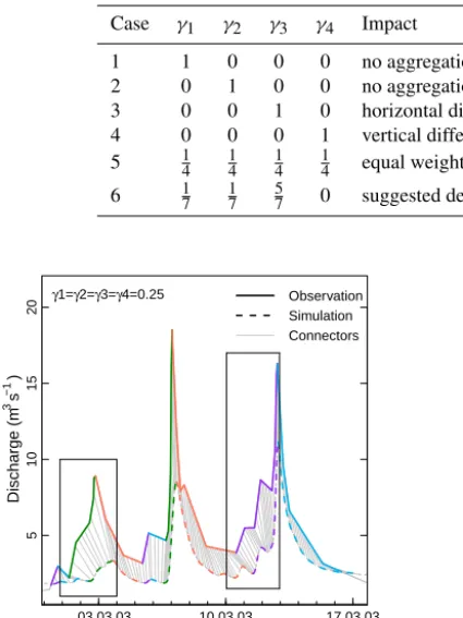
At this point the result of the SD procedure – a two-dimensional distribution of time and magnitude errors, separately for the rising and the falling segments – is available. However, in practice the problem of non-intuitive segment matching often spoils the results. Due to the constraint of time-ordered segment matching, any minor change in monotony within a rising or a falling limb that is only present in either the obs or sim event will produce a false matching of segments. The left panel in Fig. 2 illustrates this problem, where the first falling segment in the observed series (labelled with “2” in a square) corrupts segment matching: in chronolog-ical terms the steep flood rise in obs (“3” in a square) would be compared to the second rising segment in sim (“3” in a circle), which is obviously wrong. In this case, the SD time and magnitude distances will be very large, while visual comparison would most likely be done as shown in the right panel of Fig. 2 and yield good agree-ment.
We overcome this problem using iterative coarse-graining again: within the events, successively more segments are logically aggregated with their neighbours until finally the entire event consists of only two seg-ments: one rise and one fall. Compared to the last step, in which we apply coarse-graining to either sim or obs in order to equalize the number of segments in the sim-ulated and observed event, we here apply it simultane-ously to the obs and sim event. Hence, an equal number of segments and unique segment matching is ensured. The final comparison of the two events is done for the coarse-graining step in which the total SD errors and the degree of coarse-graining together are small. Both re-quirements are considered in the coarse-graining objec-tive function (θ). The latter consists of four criteria. The first two are as follows: (i) the number of edge nodes in falsely classified segments (n∗mod) and (ii) the cumu-lated importance of the dissolved segments (ISEG,cum∗ ). As discussed above, the false classifications inevitably occur during the aggregation of segments. Both cri-teria monotonically increase with the number of dis-solved segments and therefore punish excessive coarse-graining. Further criteria are (iii) the SD timing (E∗SD,t) and (iv) magnitude errors (ESD,Q∗ ) summed up over all segments of the event. They are small when segments that are hydrologically similar, i.e. close in time,
dura-tion, and magnitude, are compared. As in Eq. (1), each criterion is first normalized to the range of [0 1] and then combined using the Euclidean distance (Eq. (2)):
θ=
q
γ1n∗2mod+γ2ISEG,cum∗2 +γ3ESD,t∗2 +γ4E∗2SD,Q. (2)
Note thatθ also includes weighting factors (γ1 . . . γ4) for each criterion, which allows for a user- or time-series-specific adjustment of the objective function. Their setting is hence case-specific, with the constraint thatγ1. . . γ4have to sum up to unity. For example, if
the temporal agreement of segments is important, the weight forESD,t∗ should be large. Settingγ3=1 and all
other weights to 0 will hence result in a vertical compar-ison of the time series, provided that the positions of the edge nodes are identical. The opposite case (γ4=1 and γ1=γ2=γ3=0) minimizes vertical deviations which leads to horizontally extended SD connectors. Large weights for eitherγ1orγ2will prevent any logical ag-gregation and the pattern matching procedure will sug-gest the initial conditions as the best solution. Conse-quently, “extreme” parametrizations ofθare not mean-ingful as they will prevent the purpose of SD, which is to compare points which are hydrologically similar. As can be seen in Fig. 2, dissolving a single segment can drastically change the events’ overall SD time and mag-nitude distance. Also, as during the successive removal of segments in coarse-graining, it is impossible to pre-dict which combination of segments dissolved in obs and sim will yield the best value ofθ; thus, all possible combinations are tested and the best is kept. If, e.g., both the obs and sim event consist of 10 segments, 10×10 combinations of segment dissolutions are tested (obs1
with sim1, obs1 with sim2, etc.). The coarse-graining
scheme is thus computationally demanding. The com-bination with the minimumθ is kept and serves as the basis for the next segment reduction step in the coarse-graining procedure.
4. Once the coarse-graining is done, the optimal value ofθ
● Obs Sim
Magnitude
Time
Initial order of segments
1
●
1
2 ●
2
3 ● 3
4 ● 4
Time
Dissolved order of segments
1
●
1
[image:7.612.159.433.67.189.2]2 ● 2
Figure 2. Illustration of the time-ordered matching of segments in the coarse-graining procedure. The rising and falling segments of the
simulation (sim) and observation (obs) are numbered and colour-coded according to their chronological order. Series distance compares segments with identical number and/or colour.
03.03.03 10.03.03 17.03.03
5
10
15
20
Di
s
c
h
a
rg
e
(
m
s
)
3
−1
Date
Observation Simulation Connectors Initial conditions
03.03.03 10.03.03 17.03.03
5
10
15
20
Date Coarse-graining step=7
03.03.03 10.03.03 17.03.03
5
10
15
20
Di
s
c
h
a
rg
e
(
m
s
)
3
−1
Date Coarse-graining step=3
●
● ●
● ●
● ●
●
1 2 3 4 5 6 7
0.0
0.5
1.0
1.5
2.0
2.5
Ob
je
c
ti
v
e
f
u
n
c
ti
o
n
v
a
lu
e
(
−
)
Coarse-graining step (1=initial cond.)
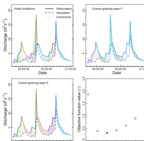
Figure 3.Coarse-graining steps: all plots contain data from the same multi-peak discharge event but for different levels of coarse-graining.
The initial conditions (top left panel) are characterized by a large number of poorly matching simulated (dashed) and observed (solid) segments as indicated by the non-intuitively placed SD connectors (grey lines). Segments required to match according to the chronological order constraint of SD are indicated by matching colours. In the last coarse-graining step (top right panel) the connectors are placed more meaningfully but the representation of the entire event by only two segments (one rise, one fall) appears inadequately coarse. The optimal level of coarse-graining, here reached at step three, yields visually acceptable connectors while preserving a detailed segment structure (bottom left panel). This step is associated with a minimum of the coarse-graining objective function (Eq. 2), indicated by the red dot in the bottom right panel. Grey dots indicated the values of the objective function for all other coarse-graining steps.
multi-peak events. The related reduction step can then be regarded as the optimal degree of coarse-graining and the final values of SD time and magnitude errors are determined based on this level. In “simple” events in which no or little coarse graining is required, the
ob-jective function values often increase fairly linearly. In any case SD time and magnitude errors are determined based upon the coarse-graining step with the smallest
[image:7.612.149.446.247.538.2]2.4 Modifications in the SD error model
In the initial version of SD, the magnitude error (ESD,Q) was calculated as the absolute difference between points in sim and obs linked by a Series Distance connector (c):
ESD,Q(c)=Qobs(c)−Qsim(c). (3)
In the current version, the magnitude error can alternatively be scaled by the mean of the connected points:
ESD,Q∗ (c)= Qobs(c)−Qsim(c)
1
2(Qobs(c)+Qsim(c))
. (4)
This yields a relative and hence dimensionless expression of the vertical error (ESD,Q∗ ), which facilitates the construction of uncertainty ranges of variable width (see Sect. 3). As in the first version of SD, both absolute and relative vertical er-ror values ESD,Q(∗) >0 indicate thatQobs(c) > Qsim(c). The
calculation of Series Distance timing errors (ESD,t)
accord-ing to Eq. (5) remained unchanged. Error values ofESD,t>0
indicate that obs occurs later than sim:
ESD,t(c)=tobs(c)−tsim(c). (5)
Similar to the scaling of the vertical error, the timing error could also be scaled using, e.g., event duration. This could be helpful if the error compared to the length of the event or the average length of all events in the time series is of interest.
The application of SD timing and magnitude error models (ESD,t(c) andESD,Q(c)) makes sense where timing errors
are both present and detectable, i.e. during events in which discharge is not constant in time. During low-flow condi-tions time offsets are, however, difficult, if not impossible to detect. Therefore, a simple one-dimensional, vertical, “stan-dard” error model analogous to Eq. (3), which relates values at the same time stept, suffices here:
ES(t )=Qobs(t )−Qsim(t ). (6)
Analogously to the scaled vertical SD error model in Eq. (4), a scaled version of the one-dimensional vertical error model (ES∗(t )) was added:
ES∗(t )= Qobs(t )−Qsim(t )
1
2(Qobs(t )+Qsim(t ))
. (7)
3 Error dressing: a heuristic approach for the construction of uncertainty ranges
The SD concept can be applied to a variety of tasks such as model diagnostics, parameter estimation, calibration, or the construction of uncertainty ranges. In this section we pro-vide one example thereof and describe a heuristic approach for the construction of uncertainty ranges for determinis-tic streamflow simulations. Uncertainty ranges provide re-gions of confidence around an uncertain estimate and are of
practical relevance and a straightforward means of highlight-ing and of assesshighlight-ing magnitude and timhighlight-ing uncertainties of hydrological simulations or forecasts. Conceptually, uncer-tainty ranges should be wide enough to capture a significant portion of the observed values but as narrow as possible to be precise and, thus, meaningful. These requirements are an-tagonistic as large uncertainty ranges, which capture most or all observations, are usually imprecise to a degree that makes them useless for decision-making purposes (Franz and Hogue, 2011).
The method we propose here follows the concept proposed by Roulston and Smith (2003) and yields quantitative esti-mates of forecast uncertainty by “dressing” single forecasts with historical error statistics. The original approach was de-signed to dress ensemble forecasts; for SD it was adapted to deterministic streamflow simulations and extended from one dimension (magnitude) to two (magnitude and timing). Like statistical approaches to uncertainty assessment, error dress-ing is based on the fundamental assumptions of ergodicity and stationarity, i.e. the assumption that errors that occurred in the past are reliable predictors for errors in the future. In the following we first outline the regular, one-dimensional deterministic error dressing method and then describe its modifications for SD.
3.1 The one-dimensional case
Provided with a record of past streamflow observa-tions (Ohist) and corresponding model simulations (Shist),
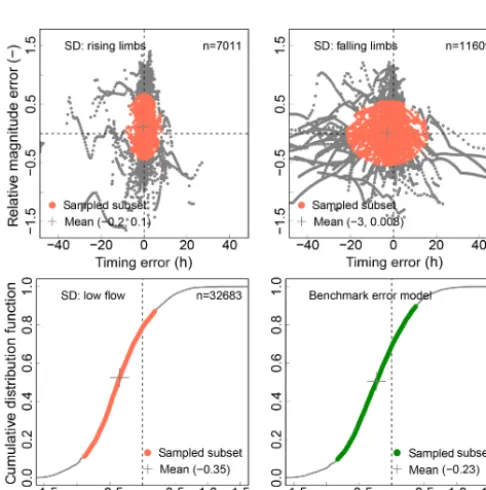
any valid error model such as Eq. (6) can be applied to calcu-late a distribution of historic errors. This distribution can then be sampled (Fig. 4, upper left panel) using a suitable strategy and the selected subset of errors can be applied to each time step of the simulation. Connecting all upper and all lower values of the dressed errors yields corresponding envelope curves (Fig. 4, upper right panel). For this procedure Roul-ston and Smith (2003) coined the term error dressing.
The choice of the sampling strategy, however, strongly influences the statistics of the resulting uncertainty ranges and should be carefully selected. In our case, the precon-dition was that the approach should be extendible to two-dimensional cases to allow its later application to the er-ror distributions of the SD approach. Therefore, we defined the sampling strategy according to the variance contribution, which is straightforward to apply for the one-dimensional case: for each point of the error distribution its relative con-tribution (dσi2) to theunbiasedvariance of the total error dis-tribution (σx2) is calculated according to Eq. (8):
dσi2=(xi−x)
2
nσ2
x
100. (8)
Herexandndenote the mean and the size of the correspond-ing error distribution. The usage of the unbiased variance, havingnin the denominator not n−1, ensures that all dσi2
ordered by the values of dσi2, and, starting with the smallest, a desired subset of all dσi2, e.g. 80 % is taken from the list. This subset represents an informal probability (p∈[0 1]) as it relates to the number of observations that fall within the un-certainty range. Small values ofpare associated with narrow (sharp) uncertainty ranges but at the cost of a higher portion of true values that fall outside. Contrary, high values of p
cause wide (imprecise) uncertainty ranges which, however, contain most errors that occurred in the past. For practical applications, typically coverages of 80 to 90 % are chosen. In Fig. 4, top left panel, the coverage was set top=0.8. 3.2 The two-dimensional case
SD yields two-dimensional distributions of coupled errors in timing and magnitude and thus requires a two-dimensional strategy for the sampling of error subsets and the construc-tion of envelope curves (Fig. 4, lower row panels).
How does one sample from bivariate distributions of cou-pled errors with different units? Statistics and computational geometry offer concepts based on the ordering of multivari-ate data sets, such as geometric median or centre point ap-proaches. The former provides a central tendency for higher dimensions and is a generalization of the median which, for one-dimensional data, has the property of minimizing the sum of distances. Centre points are generalizations of the me-dian in higher-dimensional Euclidean space and can be ap-proximated by techniques such as the Tukey depth (Tukey, 1975) or other methods of depth statistics (Mosler, 2013). Here, however, we want the errors to be centred around the mean (not around the median). Hence, we apply the same concept that we use for the one-dimensional case to SD in that we sample based on the combined contribution of each point to the total variance. Analogously to Eq. (8) we calcu-late the relative timing (dσt2) and magnitude (dσQ2) contribu-tion of each point to the total variances of the corresponding distributions. Their sum yields an estimate of the combined contribution of each point to the combined variance of both error distributions:
dσt+Q2 =dσt2+dσQ2. (9)
Analogously to the one-dimensional case, the points are ordered by increasing combined variance contribution dσt+Q2 , and, starting from the point with the smallest value which is close to or at the mean, a subset of errors can be extracted. The shape of the resulting subset depends on the underlying distribution of errors. Uncorrelated errors yield more or less circular or oval shapes (Fig. 4, lower left panel). By contrast, correlated errors yield different shapes, which is valuable for diagnostic purposes.
SD distinguishes periods of low flow, rising, and falling limbs. Hence, subsets of two 2-D error distributions (rising and falling limb) and from one one-dimensional error distri-bution (low flow) are calculated and applied to each point of
●●●●●●●●●●●●●●●●●●●●●●●●●●●●●●●●●●●●●●●●●●●●●●●●●●●●●●●●●●●●●●●●●●●●●●●●●●●●●●●●●●●●●●●●●●●●●●●●●●●●●●●●●●●●●●●●●●●●●●●●●●●●●●●●●●●●●●●●●●●●●●●●●●●●●●●●●●●●●●●●●●●●●●●●●●●●●●●●●●●●●●●●●●●●●●●●●●●●●●●●●●●●●●●●●●●●●●●●●●●●●●●●●●●●●●●●●●●●●●●●●●●●●●●●●●●●●●●●●●●●●●●●●●●●●●●●●●●●●●●●●●●●●●●●●●●●●●●●●●●●●●●●●●●●●●●●●●●●●●●●●●●●●●●●●●●●●●●●●●●●●●●●●●●●●●●●●●●●●●●●●●●●●●●●●●●●●●●●●●●●●●●●●●●●●●●●●●●●●●●●●●●●●●●●●●●●●●●●●●●●●●●●●●●●●●●●●●●●●●●●●●●●●●●●●●●●●●●●●●●●●●●●●●●●●●●●●●●●●●●●●●●●●●●●●●●●●●●●●●●●●●●●●●●●●●●●●●●●●●●●●●●●●●●●●●●●●●●●●●●●●●●●●●●●●●●●●●●●●●●●●●●●●●●●●●●●●●●●●●●●●●●●●●●●●●●●●●●●●●●●●●●●●●●●●●●●●●●●●●●●●●●●●●●●●●●●●●●●●●●●●●●●●●●●●●●●●●●●●●●●●●●●●●●●●●●●●●●●●●●●●●●●●●●●●●●●●●●●●●●●●●●●●●●●●●●●●●●●●●●●●●●●●●●●●●●●●●●●●●●●●●●●●●●●●●●●●●●●●●●●●●●●●●●●●●●●●●●●●●●●●●●●●●●●●●●●●●●●●●●● 0.0 0.2 0.4 0.6 0.8 1.0 Cu m u la ti v e d is tr ib u ti o n f u n c ti o n Vertical errors Lo w e r b o u n d a ry Up p e r b o u n d a ry Sampled subset Mean ●● ●● ● ● ● ● ● ● ● ● ● ● ● ● ● ●●● ● Discharge Time ● Simulation Envelope Sampled subset ● ● ● ● ● ● ●● ● ● ● ● ● ● ● ● ● ● ● ● ● ● ● ● ● ● ● ● ● ● ● ● ● ● ● ● ● ● ● ● ● ● ● ● ● ● ● ● ● ● ● ● ● ● ● ● ● ● ● ●● ● ● ● ● ● ● ● ● ● ● ● ● ● ● ● ● ● ● ● ● ● ● ● ● ● ● ●● ● ● ● ● ● ● ● ● ● ● ● ● ● ● ● ● ● ● ● ● ● ● ● ● ● ●● ● ● ● ● ● ● ● ● ● ● ●● ● ● ● ● ● ● ● ● ● ● ● ● ● ● ● ● ● ● ● ● ● ● ● ● ● ● ● ● ● ● ● ● ● ● ● ● ● ● ● ● ● ● ● ● ● ● ● ● ● ● ● ● ● ● ● ● ● ● ● ● ● ● ● ● ● ● ● ● ● ● ● ● ● ● ● ● ● ● ● ● ● ● ● ● ● ● ● ● ● ● ● ● ● ● ● ● ● ●● ● ● ● ● ● ● ● ● ● ● ● ● ● ● ● ● ● ● ● ● ● ● ● ● ● ● ● ● ● ● ● ● ●● ● ● ● ● ● ● ● ● ● ● ● ● ● ● ● ● ● ● ● ● ● ● ● ● ●● ● ● ● ● ● ● ● ●● ● ● ● ● ● ● ● ● ● ● ● ● ●● ● ● ● ● ● ● ● ● ● ● ● ● ● ● ● ● ● ● ● ● ● ● ● ● ● ● ● ● ● ● ● ● ● ● ● ● ● ● ● ● ● ● ● ● ● ● ● ● ● ● ● ● ● ● ● ● ● ● ● ● ● ● ● ● ● ● ● ● ● ● ● ● ● ● ● ● ● ● ● ● ● ● ● ● ● ● ● ● ● ●● ● ● ● ●● ● ● ● ● ● ● ● ● ● ● ● ● ● ● ● ● ● ● ● ● ● ● ● ● ● ● ● ● ● ● ● ● ● ● ● ● ● ● ● ● ● ● ● ● ● ● ● ● ● ● ● ● ● ● ● ● ● ● ● ● ● ● ●● ● ● ●● ● ● ● ● ● ● ● ● ● ● ● ● ● ● ● ● ● ● ● ● ● ● ● ● ● ● ● ● ● ● ● ● ● ● ● ● ● ● ● ● ● ● ● ● ● ● ● ● ● ● ● ● ● ● ● ● ● ● ● ● ● ● ● ● ● ● ● ● ● ● ● ● ● ● ● ● ● ● ● ● ● ● ● ● ● ● ● ● ● ● ● ● ● ● ● ● ● ● ● ● ●● ● ● ● ● ● ● ●● ● ● ● ● ● ● ● ● ● ● ● ● ● ● ● ● ● ● ● ● ● ● ● ● ● ● ● ●● ● ● ● ● ● ● ● ● ● ● ● ● ● ● ● ● ● ● ● ● ● ● ● ● ● ● ● ● ● ● ● ● ● ● ● ● ● ● ● ● ● ● ● ● ● ● ● ● ● ● ● ● ● ● ● ● ● ● ● ● ● ● ● ● ● ● ● ● ● ● ● ● ● ● ● ● ● ● ● ●●● ● ● ● ●● ● ● ● ● ● ● ● ● ● ● ● ● ● ● ● ● ● ● ● ● ● ● ● ● ● ● ● ● ● ● ● ● ● ● ● ● ● ● ● ● ● ● ● ● ● ● ● ● ● ● ● ● ● ● ● ● ● ● ● ● ● ● ● ● ● ● ● ● ● ● ● ● ● ● ● ● ● ● ● ● ● ● ● ● ● ● ● ● ● ● ● ● ● ● ● ● ● ● ● ● ● ● ● ● ● ● ● ● ● ● ● ● ● ● ● ● ● ● ● ● ● ● ● ● ● ● ● ● ● ● ● ● ● ● ● ● ● ● ● ● ● ● ● ● ● ● ● ● ● ● ● ● ● ●● ● ● ● ● ● ● ● ● ● ●● ● ● ● ● ● ● ● ● ● ● ● ● ● ● ● ● ● ● ● ● ● ● ● ● ● ● ● ● ● ● ● ● ● ● ● ● ● ● ● ● ● ● ● ● ● ● ● ● ● ●● ● ● ● ● ● ● ● ● ● ● ● ● ● ● ● ● ● ● ● ● ● ● ● ● ●● ● ● ● ● ● ● ● ● ● ● ● ● ● ● ● ● ● ● ● ● ● ● ● ●● ● ● ● ● ● ● ● ● ● ● ● ● ● ● ● ● ● ● ● ● ● ● ● ● ● ● ● ● ● ● ● ● ● ● ● ● ● ● ●● ● ● ● ● ● ● ● ● ● ● ● ● ● ● ● ● ● ● ● ● ● ● ● ● ● ● ● ● ● ● ● ● ● ● ● ● ● ● ● ● ● ● ● ● ●● ● ● ● ● ● ● ● ● ● ● ● ● ● ● ● ● ● ● ● ●● ● ● ● ● ● ● ● ● ● ● ● ● ● ● ● ● ● ● ● ● ● ● ●● ● ● ● ● ● ● ● ● ●● ● ● ● ● ● ● ● ● ● ● ● ● ● ● ● ● ● ● ● ● ● ● ● ● ● ● ● ● ● ● ● ● ● ● ● ● ● ● ● ● ● ● ● ● ● ● ● ● ● ● ● ● ● ● ● ● ● ● ● ● ● ● ● ● ● ●● ● ● ● ● ● ●● ● ● ●● ● ● ● ● ● ● ● ● ● ● ● ● ● ● ● ● ● ● ● ● ● ● ● ● ● ● ● ●● ● ● ● ● ● ● ● ● ● ● ● ● ● ● ● ●● ● ● ● ● ● ● ●● ● ● ● ● ● ● ● ● ● ● ●● ● ● ● ● ● ● ● ● ● ● ● ● ● ● ● ● ● ● ● ● ● ● ● ● ● ● ● ● ● ● ● ● ● ● ● ● ● ● ● ● ● ● ● ● ● ● ● ● ● ● ● ● ● ● ● ● ● ● ● ● ● ● ● ● ● ● ● ● ● ● ●● ● ● ● ●● ● ● ● ● ● ● ● ● ● ● ● ● ● ● ● ● ● ● ● ● ● ● ● ● ● ● ● ● ● ● ● ● ● ● ● ● ● ● ● ● ● ● ● ● ● ● ● ●● ● ●●● ● ● ● ● ● ● ● ● ● ● ● ● ● ● ● ● ●● ● ● ● ● ● ● ● ● ● ● ● ● ● ● ● ● ● ● ● ● ● ● ● ● ● ● ● ● ● ● ● ● ● ● ● ● ● ● ● ● ● ● ● ● ● ● ● ● ● ● ● ● ● ● ● ● ● ● ● ● ● ●● ● ● ● ● ●● ● ● ● ● ● ● ● ● ● ● ● ● ● ● ● ● ● ● ●● ● ● ● ● ●● ● ● ● ● ● ● ● ● ● ● ● ● ● ● ● ● ● ● ● ● ● ● ● ● ● ● ● ● ● ● ● ● ● ● ● ● ● ● ● ● ● ● ● ● ● ● ● ● ● ● ● ● ● ● ● ● ● ● ● ● ● ● ● ● ● ● ●● ● ● ● ● ●● ● ● ● ● ● ● ● ● ● ● ● ● ● ● ● ● ● ● ● ● ● ● ● ● ● ● ● ● ● ● ● ● ● ● ● ● ● ● ● ● ● ● ● ● ● ● ● ● ● ● ● ● ● ● ● ● ● ● ● ● ● ● ● ● ● ● ● ● ● ● ● ● ● ● ● ● ● ● ● ● ● ● ● ● ● ● ● ● ● ● ● ● ● ● ● ● ● ● ● ● ● ● ● ● ● ● ● ● ● ● ● ● ● ● ● ●● ● ● ● ● ● ● ● ● ● ●● ● ● ● ● ● ● ● ● ● ● ● ● ● ● ● ● ● ● ● ● ● ● ● ● ● ● ● ● ● ● ● ● ● ● ● ● ● ●● ● ● ● ● ● ● ● ● ● ● ● ● ● ● ● ● ● ● ●● ● ● ● ● ● ● ● ● ● ● ● ● ● ● ● ● ●● ● ● ● ● ● ● ● ● ● ● ● ● ● ● ● ● ● ● ● ● ● ● ● Magnitude error Timing error
● Sampled subset
Means
●
●
Highest dσt+Q2 Smallest dσt+Q2
●●● ● ● ● ● ●● ● ● ● ● ● ● ● ●● ● ● ●●●●● ● ● ●●● ● ●● ● ● ● ● ●●● ● ● ● ● ● ● ● ● ● ● ●● ● ●● ● ● ● ● ● ● ● ● ● ● ● ● ●●●● ● ● ● ●● ● ● ● ● ● ●● ● ● ● ● ● ● ● ● ● ● ● ● ● ● ● ●● ● ● ● ● ● ● ● ● ●●● ● ● ● ● ● ● ● ●● ● ●●● ● ● ● ● ● ● ● ● ● ● ● ● ● ●● ●●● ● ● ● ● ● ● ●● ● ● ● ● ●● ● ● ●● ● ● ● ● ● ● ●● ● ● ● ● ● ● ●●●● ● ● ● ● ●● ●● ●● ● ● ● ● ● ● ● ● ● ● ● ●●●● ● ● ● ● ●● ● ● ● ●● ●●● ● ● ● ● ●●● ● ● ● ● ● ● ● ●●● ● ● ●●● ● ●● ● ● ● ● ● ● ●● ● ●●● ● ● ● ● ● ● ● ● ● ● ● ● ● ● ● ●●●● ● ● ● ● ●● ● ● ● ●● ● ● ● ● ● ● ● ● ● ● ●● ● ● ●● ● ● ● ● ● ● ● ● ● ● ● ● ● ● ● ●● ● ● ● ● ● ●● ●● ● ● ● ●● ● ● ● ●● ● ●●● ● ● ● ● ● ●●● ● ● ●● ● ● ● ● ● ● ● ● ● ● ● ● ● ●● ● ● ● ● ● ● ●● ● ● ● ●● ● ●● ● ● ● ● ● ● ● ● ● ● ● ● ● ● ● ●● ●● ● ● ● ●● ●● ● ● ● ● ● ● ● ● ● ● ● ●● ● ● ● ● ● ● ● ● ● ● ● ● ● ● ● ● ● ● ● ● ● ● ● ● ● ●● ● ● ● ● ● ● ● ● ● ● ●● ● ● ● ● ● ● ● ● ● ● ● ● ●● ● ● ●● ●●● ● ● ●● ● ● ●●●● ● ●●●● ●● ●●● ●● ● ● ● ● ● ● ● ●● ● ● ● ● ● ●● ● ● ● ● ● ● ● ● ● ● ● ● ● ● ● ● ● ● ● ●● ● ● ● ● ● ● ● ●●● ● ● ● ●● ●● ● ● ● ● ● ●● ● ● ● ● ●● ● ● ● ● ●●● ● ● ● ● ● ● ● ● ●● ● ● ● ● ●●●● ● ● ●●● ● ● ● ● ●●● ● ● ● ● ● ● ●● ● ● ● ●● ● ● ● ● ● ● ● ● ● ● ● ● ●●● ● ● ● ● ● ● ● ● ●● ● ● ● ● ● ● ● ● ● ● ● ● ● ● ● ● ● ● ● ● ● ● ● ● ● ● ● ● ●● ● ●● ● ● ● ● ● ● ● ●● ● ● ● ●● ● ● ●●●● ● ● ● ● ● ● ● ● ● ● ● ●● ●●●● ● ● ● ● ● ● ● ● ● ● ● ● ● ● ● ● ●● ● ●●● ● ● ●● ● ● ● ● ● ●●● ● ● ● ● ●●●●●●●●● ● ● ●● ● ●● ● ● ● ● ●● ● ● ● ● ● ● ● ● ● ● ● ● ● ● ● ● ● ● ● ●● ● ● ●●● ● ● ● ● ●● ● ● ● ● ● ● ● ●● ● ● ●●●●● ● ● ●●● ● ●● ● ● ● ● ●●● ● ● ● ● ● ● ● ● ● ● ●● ● ●● ● ● ● ● ● ● ● ● ● ● ● ● ●●● ● ● ● ● ●● ● ● ● ● ● ●● ● ● ● ● ● ● ●● ● ● ● ● ● ● ● ●● ● ● ● ● ● ● ● ● ●●● ● ●● ● ● ● ● ●● ● ●●● ● ● ● ● ● ● ● ● ● ● ● ● ● ●● ●●● ● ● ● ● ●●●● ● ● ● ● ●● ● ● ●● ● ● ● ● ● ● ●● ● ● ● ● ● ● ●●●● ● ● ● ● ●● ●● ●● ● ● ● ● ● ● ● ● ● ● ● ●●●● ● ● ● ● ●● ● ● ● ●● ●●● ● ● ● ● ●●● ● ● ● ● ● ● ● ●● ● ● ● ●●● ● ●● ● ● ● ● ● ● ●● ● ●●● ● ● ● ● ● ● ● ● ● ● ● ● ● ● ● ●●●● ● ● ● ● ●● ● ● ● ●● ● ● ● ● ● ● ● ● ● ● ●● ● ● ●● ● ● ● ● ● ● ● ● ● ● ● ● ● ● ● ●● ● ● ● ● ● ●● ●● ● ● ● ●● ● ● ● ●● ● ●●● ● ● ● ● ● ●●● ● ● ●● ● ● ● ● ● ● ● ● ● ● ● ● ● ●● ● ● ● ● ● ● ●● ● ● ● ●● ● ●● ● ● ● ● ● ● ● ● ● ● ● ● ● ● ● ●● ●● ● ● ● ●● ●● ● ● ● ● ● ● ● ● ● ● ● ●● ● ● ● ● ● ● ● ● ● ● ● ● ● ● ● ● ● ● ● ● ● ● ● ● ● ●● ● ● ● ● ● ● ● ● ● ● ●● ● ● ● ● ● ● ● ● ● ● ● ● ●● ● ● ●● ●●● ● ● ●● ● ● ●●●● ● ●●●● ●● ●●● ●● ● ● ● ● ● ● ● ●● ● ● ● ● ● ●● ● ● ● ● ● ● ● ● ● ● ● ● ● ● ● ● ● ● ● ● ● ● ● ● ● ● ● ● ●●● ● ● ● ●● ●● ● ● ● ● ● ●● ● ● ● ● ●● ● ● ● ● ●●● ● ● ● ● ● ● ● ● ●● ● ● ● ● ●●●● ● ● ●●● ● ● ● ● ●●● ● ● ● ● ● ● ●● ● ● ● ●● ● ● ● ● ● ● ● ● ● ● ● ● ●●● ● ● ● ● ● ● ● ● ●● ● ● ● ● ● ●●● ● ● ● ● ● ●● ● ● ● ● ● ● ● ● ● ● ● ● ● ●● ● ●● ● ● ● ● ● ● ● ●● ● ● ● ●● ● ● ●●●● ● ● ● ● ● ● ● ● ● ● ● ● ● ●●●● ● ● ● ● ● ● ● ● ● ● ● ● ● ● ● ● ●● ● ●●● ● ● ●● ● ● ● ● ● ●●● ● ● ● ● ●●●●●●●●● ● ● ●● ● ●● ● ● ●● ●● ● ● ● ● ● ● ● ● ● ● ● ● ● ● ● ● ● ● ● ●● ● ● ●●●● ● ● ● ●● ● ● ● ● ● ● ● ●● ● ● ●●●●● ● ● ●●● ● ● ● ● ● ● ● ● ●● ● ● ● ● ● ● ● ● ● ● ●● ● ●● ● ● ● ● ● ● ● ● ●● ● ● ●●● ● ● ● ● ●● ● ● ● ● ● ●● ● ● ● ● ● ● ●● ● ● ● ● ● ● ● ●● ● ● ● ● ● ● ● ● ●●● ● ●● ● ● ● ● ●● ● ●●● ● ● ● ● ● ● ● ● ● ● ● ● ● ●● ●●● ● ● ● ● ●●●● ● ● ● ● ●● ● ● ●● ● ● ● ● ● ● ●● ● ● ● ● ● ● ●●●● ● ● ● ● ●● ●● ●● ●● ● ● ● ● ● ● ● ● ● ●●●● ● ● ● ● ●● ● ● ● ●● ●●● ● ● ● ● ●●● ● ● ● ● ● ● ● ●● ● ● ● ●●● ● ●● ● ● ● ● ● ● ●● ● ●●● ● ● ● ● ● ● ● ● ● ● ● ● ● ● ● ●●●● ● ● ● ● ●● ● ● ● ●● ● ● ● ● ● ● ● ● ● ● ●● ● ● ●● ● ● ● ● ● ● ● ● ● ● ● ● ● ● ● ●● ● ● ● ● ● ●● ●● ● ● ● ●● ● ● ● ●● ● ●●● ● ● ● ● ● ●●● ● ● ● ● ● ● ● ● ● ● ● ● ● ● ● ● ● ●● ● ● ● ● ● ● ●● ● ● ● ●● ● ●● ● ● ● ● ● ● ● ● ● ● ● ● ● ● ● ●● ●● ● ● ● ●● ●● ● ● ● ● ● ● ● ● ● ● ● ●● ● ● ● ● ● ● ● ● ● ● ● ● ● ● ● ● ● ● ● ● ● ● ● ● ● ●● ● ● ● ● ● ● ● ● ● ●●●● ● ● ● ● ● ● ● ● ● ● ● ●● ● ● ●● ●●● ● ● ●● ● ● ●●●● ● ● ●●● ●● ●●● ●● ● ● ● ● ● ● ● ●● ● ● ● ● ● ●● ● ● ● ● ● ● ● ● ● ● ● ● ● ● ● ● ● ● ● ● ● ● ● ● ● ● ● ● ●●● ● ● ● ●● ●● ● ● ● ● ● ●● ● ● ● ● ●● ● ● ● ● ●●● ● ● ● ● ● ● ● ● ●● ● ● ● ● ●●●● ● ● ●●● ● ● ● ● ●●● ● ● ● ● ● ● ●● ● ● ● ●● ● ● ● ● ● ● ● ● ● ● ● ● ●●● ● ● ● ● ● ● ● ● ●● ● ● ● ● ● ●●● ● ● ● ● ● ●● ● ● ● ● ● ● ● ● ● ● ● ● ● ●● ● ●● ● ● ● ● ● ● ● ●● ● ● ● ●● ● ● ●●●● ● ● ● ● ● ● ● ● ● ● ● ● ● ●●●● ● ● ● ● ● ● ● ● ● ● ● ● ● ● ● ● ●● ● ●●● ● ● ●● ● ● ● ● ● ●●● ● ● ● ● ●●●●●●●●● ● ● ●● ● ●● ● ● ●● ●● ● ● ● ● ● ● ● ● ● ● ● ● ● ● ● ● ● ● ● ●● ● ● ●●● ● ● ● ● ●● ● ● ● ● ● ● ● ●● ● ● ●●●●● ● ● ●●● ● ●● ● ● ● ● ● ●● ● ● ● ● ● ● ● ● ● ● ●● ● ●● ● ● ● ● ● ● ● ● ●● ● ● ●●● ● ● ● ● ●● ● ● ● ● ● ●● ● ● ● ● ● ● ●● ● ● ● ● ● ● ● ●● ● ● ● ● ● ● ● ● ●●● ● ●● ● ● ● ● ●● ● ●●● ● ● ● ● ● ● ● ● ● ● ● ● ● ●● ●●● ● ● ● ● ●●●● ● ● ● ● ●● ● ● ●● ● ● ● ● ● ● ●● ● ● ● ● ● ● ●●●● ● ● ● ● ●● ●● ●● ● ● ● ● ● ● ● ● ● ● ● ●●●● ● ● ● ● ●● ● ● ● ●● ●●● ● ● ● ● ●●● ● ● ● ● ● ● ● ●● ● ● ● ●●● ● ●● ● ● ● ● ● ● ●● ● ●●● ● ● ● ● ● ● ● ● ● ● ● ● ● ● ● ●●●● ● ● ● ● ●● ● ● ● ●● ● ● ● ● ● ● ● ● ● ● ●● ● ● ●● ● ● ● ● ● ● ● ● ● ● ● ● ● ● ● ●● ● ● ● ● ● ●● ●● ● ● ● ●● ● ● ● ●● ● ●●● ● ● ● ● ● ●●● ● ● ●● ● ● ● ● ● ● ● ● ● ● ● ● ● ●● ● ● ● ● ● ● ●● ● ● ● ●● ● ●● ● ● ● ● ● ● ● ● ● ● ● ● ● ● ● ●● ●● ● ● ● ●● ●● ● ● ● ● ● ● ● ● ● ● ● ●● ● ● ● ● ● ● ● ● ● ● ● ● ● ● ● ● ● ● ● ● ● ● ● ● ● ●● ● ● ● ● ● ● ● ● ● ● ●● ● ● ● ● ● ● ● ● ● ● ● ● ●● ● ● ●● ●●● ● ● ●● ● ● ●●●● ● ● ●●● ●● ●●● ●● ● ● ● ● ● ● ● ●● ● ● ● ● ● ●● ● ● ● ● ● ● ● ● ● ● ● ● ● ● ● ● ● ● ● ● ● ● ● ● ● ● ● ● ●●● ● ● ● ●● ●● ● ● ● ● ● ●● ● ● ● ● ●● ● ● ● ● ●●● ● ● ● ● ● ● ● ● ●● ● ● ● ● ●●●● ● ● ●●● ● ● ● ● ●●● ● ● ● ● ● ● ●● ● ● ● ●● ● ● ● ● ● ● ● ● ● ● ● ● ●●● ● ● ● ● ● ● ● ● ●● ● ● ● ● ● ●●● ● ● ● ● ● ●● ● ● ● ● ● ● ● ● ● ● ● ● ● ●● ● ●● ● ● ● ● ● ● ● ●● ● ● ● ●● ● ● ●●●● ● ● ● ● ● ● ● ● ● ● ● ● ● ●●●● ● ● ● ● ● ● ● ● ● ● ● ● ● ● ● ● ●● ● ●●● ● ● ●● ● ● ● ● ● ●●● ● ● ● ● ●●●●●●●●● ● ● ●● ● ●● ● ● ●● ●● ● ● ● ● ● ● ● ● ● ● ● ● ● ● ● ● ● ● ● ●● ● ● ●●● ● ● ● ● ●● ● ● ● ● ● ● ● ●● ● ● ●●●●● ● ● ●● ● ● ●● ● ● ● ● ●●● ● ● ● ● ● ● ● ● ● ● ●● ● ●● ● ● ● ● ● ● ● ● ● ● ● ● ●●●● ● ● ● ●● ● ● ● ● ● ●● ● ● ● ● ● ● ● ● ● ● ● ● ● ● ● ●● ● ● ● ● ● ● ● ● ●●● ● ● ● ● ● ● ● ●● ● ●●● ● ● ● ● ● ● ● ● ● ● ● ● ● ●● ●●● ● ● ● ● ● ● ●● ● ● ● ● ●● ● ● ●● ● ● ● ● ● ● ●● ● ● ● ● ● ● ●●●● ● ● ● ● ●● ●● ●● ● ● ● ● ● ● ● ● ● ● ● ●●●● ● ● ● ● ●● ● ● ● ●● ●●● ● ● ● ● ●●● ● ● ● ● ● ● ● ●●● ● ● ●●● ● ●● ● ● ● ● ● ● ●● ● ●●● ● ● ● ● ● ● ● ● ● ● ● ● ● ● ● ●●●● ●●● ● ●● ● ● ● ●● ● ● ● ● ● ● ● ●● ● ●● ● ● ●● ● ● ● ● ● ● ● ● ● ● ● ● ● ● ● ●● ● ● ● ●● ●● ●● ● ● ● ●● ● ● ● ●● ● ●●● ● ● ● ● ● ●●● ● ● ●● ● ● ● ● ● ● ● ● ● ● ● ● ● ● ● ● ● ● ● ● ● ●● ● ● ● ●● ● ●● ● ● ● ● ● ● ● ● ● ● ● ● ● ● ● ●● ●● ● ● ● ●● ●● ● ● ● ● ● ● ● ● ● ● ● ●● ● ● ● ● ● ● ● ● ● ● ● ● ● ● ● ● ● ● ● ● ● ● ● ● ● ●● ● ● ● ● ● ● ● ● ● ●●●● ● ● ● ● ● ● ● ● ● ● ● ●● ● ● ●● ●●● ●●●● ● ● ●●●● ● ● ●●● ● ● ●●● ●● ● ● ● ● ● ● ● ●● ● ● ● ● ● ●● ● ● ● ● ● ● ● ● ● ● ● ● ● ● ● ● ● ● ● ●● ● ● ● ● ● ● ● ●●● ● ● ● ●● ●● ● ● ● ● ● ●● ● ● ● ● ●● ● ● ● ● ●●● ● ● ● ● ● ● ● ● ●● ● ● ● ● ●●●● ● ● ●●● ● ● ● ● ●●● ● ● ● ● ● ● ●● ● ● ● ●● ● ● ● ● ● ● ● ● ● ● ● ● ●●● ● ● ● ● ● ● ● ● ●● ● ● ● ● ● ● ● ● ● ● ● ● ● ● ● ● ● ● ● ● ● ● ● ● ● ● ● ● ●● ● ●● ● ● ● ● ● ● ● ●● ● ● ● ● ● ● ● ●●●● ● ● ● ● ● ● ● ● ● ● ● ●● ●●●● ● ● ● ● ● ● ● ● ● ● ● ● ● ● ● ● ●● ● ●●● ● ● ●● ● ● ● ● ● ●●●●● ● ● ●●●●●●●●● ● ● ●● ● ●● ● ● ● ● ●● ● ● ● ● ● ● ● ● ● ● ● ● ● ● ● ● ● ● ● ●● ● ● ●●●● ● ● ● ●● ● ● ● ● ● ● ● ●● ● ● ●●●●● ● ● ●●● ● ● ● ● ● ● ● ● ●● ● ● ● ● ● ● ● ● ● ● ●● ● ●● ● ● ● ● ● ● ● ● ● ● ● ● ●●●● ● ● ● ●● ● ● ● ● ● ●● ● ● ● ● ● ● ● ● ● ● ● ● ● ● ● ●● ● ● ● ● ● ● ● ● ●●● ● ● ● ● ● ● ●●●● ●●● ● ● ● ● ● ● ● ● ● ● ● ● ● ●● ●●●● ● ● ● ● ● ●● ● ● ● ● ●● ● ● ●● ● ● ● ● ● ● ●● ● ● ● ● ● ● ●●●● ● ● ● ● ●● ●● ●● ● ● ● ● ● ● ● ● ● ● ● ●●●● ● ● ● ● ●● ● ● ● ●● ●●● ● ● ● ● ●●● ● ● ● ● ● ● ● ●● ● ● ● ●●● ● ●● ● ● ● ● ● ● ●● ● ●●● ● ● ● ● ● ● ● ● ● ● ● ● ● ● ● ●●●● ●●● ● ●● ● ● ● ●● ● ● ● ● ● ● ● ●● ● ●● ● ● ●● ● ● ● ● ● ● ● ● ● ● ● ● ● ● ● ●● ● ● ● ●● ●● ●● ● ● ● ●● ● ● ● ●● ● ●●● ● ● ● ● ● ●●● ● ● ●● ● ● ● ● ● ● ● ● ● ● ● ● ● ●● ● ● ● ● ● ● ●● ● ● ● ●● ● ●● ● ● ● ● ● ● ● ● ● ● ● ● ● ● ● ●● ●● ● ● ● ● ● ●● ● ● ● ● ● ● ● ● ● ● ● ●● ● ● ● ● ● ● ● ● ● ● ● ● ● ● ● ● ● ● ● ● ● ● ● ● ● ●● ● ● ● ● ● ● ● ● ● ●●●● ● ● ● ● ● ● ● ● ● ● ● ●● ● ● ●● ●●● ●●●● ● ● ●●●● ● ● ●●● ● ● ●●● ●● ● ● ● ● ● ● ● ●● ● ● ● ● ● ●● ● ● ● ● ● ● ● ● ● ● ● ● ● ● ● ● ● ● ● ● ● ● ● ● ● ● ● ● ●●● ● ● ● ● ● ●● ● ● ● ● ● ●● ● ● ● ● ●● ● ● ● ● ●●● ● ● ● ● ● ● ● ● ●● ● ● ● ● ●●●● ● ● ●●● ● ● ● ● ●●● ● ● ● ● ● ● ●● ● ● ● ●● ● ● ● ● ● ● ● ● ● ● ● ● ●●● ● ● ● ● ● ● ● ● ●● ● ● ● ● ● ● ● ● ● ● ● ● ● ● ● ● ● ● ● ● ● ● ● ● ● ● ● ● ●● ● ●●● ● ● ● ● ● ● ●● ● ● ● ●● ● ● ●●●● ● ● ● ● ● ● ● ● ● ● ● ● ● ●●●● ● ● ● ● ● ● ● ● ● ● ● ● ● ● ● ● ●● ● ●● ● ● ● ●● ● ● ● ● ● ●●●●● ● ● ●●●●●●●●● ● ● ●● ● ●● ● ● ●● ●● ● ● ● ● ● ● ● ● ● ● ● ● ● ● ● ● ● ● ● ●● ● ● ● ●● ● ● ● ● ● ● ● ●● ● ● ● ● ● ●● ●● ● ● Simulation Envelope Sampled subset Discharge Time
Figure 4.Sketch of the one- and two-dimensional error dressing
method using normally distributed random numbers (n=1000). The upper row panels show the one-dimensional case with an em-pirical cumulative distribution function of errors (upper left panel) and an 80 % subset thereof sampled according to increasing vari-ance contribution. The application (dressing) of the subset of errors to a hydrograph and the construction of the corresponding envelop curves is illustrated in the upper right panel. The lower row pan-els show the same procedure for the two-dimensional case. From the two-dimensional distribution of empirical errors (bottom left panel) 80 % (colour-coded) are again sampled according to the com-bined variance contribution of both distributions (colour ramp). The bottom right panel contains a sketch of the two-dimensional error dressing method and the construction of envelope curves. Please note that the use of normally distributed numbers yields symmetri-cal samples and envelopes, which is usually not the case for real-world data, which are usually skewed.
4 Case study
This case study, based on real-world data, serves to present and to discuss relevant aspects of SD by comparison with a benchmark error model (BM).
4.1 Data and site properties
We used discharge observations (Ohist) of a 6-year
pe-riod (30 October 1999–30 October 2005) from gauge “Ho-her Steg” (HOST), which is located in the small alpine catchment of the Dornbirner Ach River in north-western Austria. Catchment size is 113 km2, the elevation range is 400–2000 m a.s.l., and mean annual rainfall differs between 1100 and 2100 mm yr−1. For the 6-year period, hourly hy-drometeorological time series (n=52 633 time steps) were used to drive an existing, calibrated conceptual water bud-get model of the type LARSIM (Large Area Runoff Simu-lation Model, gridded version, resolution=1 km2; Ludwig and Bremicker, 2006), which yielded acceptable simula-tions (Shist) with a NASH of 0.78. Please note that for the
discussion of the SD concept, neither the model itself nor the catchment properties are particularly relevant. The main purpose of the case study was to apply realistic data. This is also the reason why we used the entire 6-year period to both derive and apply the error distributions; i.e. we did not distinguish periods of error analysis and error application. 4.2 Conceptual setup
For the benchmark model, we derived distributions of 1-D vertical errors. We did not differentiate cases of low flow and events, which is rather simplistic but standard practice. For the SD approach we did differentiate these cases. This may be considered an unfair advantage for SD as it allows the construction of more custom-tailored uncertainty envelopes. However, as the objective of the case study is not a compe-tition between the two approaches but a way to present in-teresting aspects of SD, we considered it justified. For SD, the required starting and end points of hydrological events were manually determined both in Ohist andShist by visual
inspection. Altogether there weren=123 events in each se-ries, and they were fully matching; i.e. no missing events or false alarms occurred. The resulting contingency table is ob-viously trivial and therefore not discussed further here.
Both for SD and BM, we applied scaled errors (ESD,Q∗ (c)
according to Eq. (4) andEBMaccording to Eq. (7), respec-tively), as we found that compared to the standard error model, they are more applicable across the usually large dis-charge ranges present in hydrographs. For SD, the weights
γ1, . . . , γ4 used in the objective function of the
coarse-graining procedure (Eq. 2) were set to17,17,57, and 0, respec-tively, based on iteratively maximizing the visual agreement of segments in matching events of sim and obs. Additional studies with different data sets (not shown here) yielded
sim-ilar optimal weights, which corroborates that this is a rel-atively robust choice and sufficient for a proof of concept, as intended in this study. For more widespread applications, a detailed sensitivity analysis is desirable. Such an analy-sis is, however, difficult as several different time series, flow conditions, and rainfall–runoff events would have to be vi-sualized and compared. Moreover, there is no robust bench-mark available to which we may compare the outcome of the proposed coarse-graining procedure. For this reason we provide software such that any interested person can find out for him/herself whether the proposed method suits his or her needs or not.
Based upon SD and BM we derived empirical error dis-tributions from the entire test period and then used them, in the same period, to construct uncertainty envelopes around the simulation Shist using the error dressing approach as described in Sect. 3. To ensure comparability we enforced identical coverages for both approaches during the construc-tion of the envelope curves; i.e. we made sure that the de-sired fraction of observations (e.g. 80 %) fell within the un-certainty envelope. For the standard error model this was straightforward: if from the 1-D distribution of errors a subset ofp=80 % is selected and used to construct the uncertainty envelope as described in Sect. 3.1 for the same period of time, then by definition the number of observations within the en-velope must also be 80 %. For SD, however, as a consequence of error ovals overlapping in time (Fig. 4, lower right panel), this is not self-evident and typically many more observations fall within the uncertainty envelope than the levelpat which the subset of the 2-D error distribution is sampled. This issue was solved by iteratively sampling the error distributions at various levels ofpuntil the desired percentage of observa-tions (here: 80 %) fell within the uncertain envelope. 4.3 Evaluation of deterministic uncertainty ranges The evaluation of deterministic uncertainty ranges requires methods to quantify properties such as coverage or precision. Here we propose a set of statistics which can be applied to uncertainty ranges irrespective of how they were constructed. While this ensures comparability of the SD and BM-derived ranges, it does not exploit the advantages of the SD approach, i.e. separate treatment of time and magnitude uncertainties.
1. Coverage (φ) is the most intuitive criterion. It quantifies the ratio of observations that fall inside the simulated uncertainty range and can take values between 0 (no single observed value included) and 1 (all observations included). φ can easily be obtained as the number of observations (nobs) that fall inside the uncertainty range around a simulation, divided by the total length of the time series (n):
φ=nobs