Cascade based disaggregation of continuous rainfall time series: the influence of climate

Cascade-based disaggregation of continuous rainfall time series:

the influence of climate

Andreas Güntner

_{*, Jonas Olsson}

_{, Ann Calver}

_{and Beate Gannon}

1_{Potsdam Institute for Climate Impact Research, P.O. Box 601203, 14412 Potsdam, Germany}

2_{Institute of Environmental Systems (SUIKO), Kyushu University, 6-10-1 Hakozaki, Higashi-ku, Fukuoka 812-8581, Japan; currently at: Department of Water Resources}

Engineering, Lund University, Box 118, SE-221 00 Lund, Sweden

3_{CEH, Wallingford, Oxfordshire, OX10 8BB, UK}

*Email for corresponding author: [email protected]

Abstract

Rainfall data of high temporal resolution are required in a multitude of hydrological applications. In the present paper, a temporal rainfall disaggregation model is applied to convert daily time series into an hourly resolution. The model is based on the principles of random multiplicative cascade processes. Its parameters are dependent on (1) the volume and (2) the position in the rainfall sequence of the time interval with rainfall to be disaggregated. The aim is to compare parameters and performance of the model between two contrasting climates with different rainfall generating mechanisms, a semi-arid tropical (Brazil) and a temperate (United Kingdom) climate. In the range of time scales studied, the scale-invariant assumptions of the model are approximately equally well fulfilled for both climates. The model parameters differ distinctly between climates, reflecting the dominance of convective processes in the Brazilian rainfall and of advective processes associated with frontal passages in the British rainfall. In the British case, the parameters exhibit a slight seasonal variation consistent with the higher frequency of convection during summer. When applied for disaggregation, the model reproduces a range of hourly rainfall characteristics with a high accuracy in both climates. However, the overall model performance is somewhat better for the semi-arid tropical rainfall. In particular, extreme rainfall in the UK is overestimated whereas extreme rainfall in Brazil is well reproduced. Transferability of parameters in time is associated with larger uncertainty in the semi-arid climate due to its higher interannual variability and lower percentage of rainy intervals. For parameter transferability in space, no restrictions are found between the Brazilian stations whereas in the UK regional differences are more pronounced. The overall high accuracy of disaggregated data supports the potential usefulness of the model in hydrological applications.

Keywords: Rainfall, temporal disaggregation, random cascade, scaling, semi-arid, temperate climate.

Introduction

The access to high-resolution temporal rainfall data is of prime importance in a multitude of hydrological applications including rainfall-runoff and water balance modelling, flood forecasting and computer models of pollutant transport. The serious floods in Europe and elsewhere during recent years, whether related to the rainfall regime or to changes in the land use, emphasise the importance of assessing accurately short-term processes of runoff generation. For basin-scale applications, traditionally a daily time step has been used in hydrological models. Particularly for modelling flood flows, however, rainfall time series of higher resolution are required, since high rainfall intensities over short periods frequently have a significant effect on peak flows and flood frequency curves. While daily data are usually available,

1996). In a flood modelling context, one of few approaches employed is the so-called average variability method (Pilgrim et al., 1969; Lamb and Calver, 1998).

A novel approach to model the statistical distribution of rainfall in time and space that has emerged during the eighties and nineties is by random cascade processes (e.g. Schertzer and Lovejoy, 1987). In the sense used here, a cascade process repeatedly divides the available space (of any dimension) into smaller regions, in each step re-distributing some associated quantity according to rules specified by the so-called cascade generator. Originating as a turbulent kinetic energy model (e.g. Yaglom, 1966), this concept was proposed to reproduce the empirically observed scaling behaviour of rainfall (e.g. Gupta and Waymire, 1990). In general, scaling may be defined as a log-log linear relationship between statistical moments of various orders and a scale parameter. This behaviour is a generic feature of random cascades. Concerning the presence of scaling and applicability of cascade models to temporal rainfall, this has been supported in a number of empirical data analyses (e.g. Hubert et al., 1993; Olsson, 1995; Harris et al., 1996; Svensson et al., 1996; Tessier et al., 1996). With regard to temporal rainfall modelling, this has been performed mainly by calibrating the general so-called universal multifractal model (e.g. Lovejoy and Schertzer, 1990) on rainfall time series (e.g. Hubert et al., 1993; Olsson et al., 1993; Tessier

et al., 1993, 1996; de Lima and Grasman, 1999), but other

random cascade models have also been employed (e.g. Menabde et al., 1997, 1999; Deidda et al., 1999).

Olsson (1998) developed a cascade-based model for continuous rainfall time series. The model combined an underlying hypothesis of cascade-type scaling with empirically observed features of temporal rainfall. Besides the more simplistic and applied nature of the model, the main difference compared with other approaches was the assumption of a dependency between the cascade generator and two properties of the time series values, namely rainfall volume and position in the rainfall sequence. This assumption was supported in an analysis of a rainfall time series from southern Sweden, and the model was shown to be applicable between approximately 1 week and 1 hour. After calibration, the model was used for disaggregation from approximately 16 hours to 1 hour. Despite being built solely upon scaling properties, the model reproduced not only the scaling behaviour of the observed data, but also the intermittent nature and the distributional properties of both individual volumes and event-related measures.

The purpose of the present study is to develop further and test the model with various objectives, the main one being to assess the performance in different climate regimes. Specifically, it is intended to evaluate the value of the

cascade scheme for representing and disaggregating rainfall in two different climates, and to relate both model parameters and the accuracy of generated data to regional meteorological characteristics. Other aims include assessments of extreme value performance, parameter transferability in space and time, and disaggregation in the specific range 1 day to 1 hour, a scale range of high practical relevance.

Rainfall data

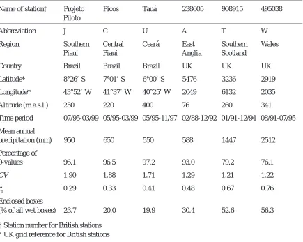
As an example of a semi-arid climate, rainfall data of three stations in north-eastern Brazil were analysed (Table 1). The rainfall regime in the study area is characterised by a rainy season with duration of about five months and maximum precipitation in March or April. The principal mechanisms generating rainfall are: (1) The Intertropical Convergence Zone which migrates seasonally, reaching its southernmost position in March, (2) cold fronts and their remnants from high latitudes of the southern hemisphere, (3) tropical meso-scale mechanisms, like upper tropospheric cyclonic vortices, land-sea circulations and topography-driven meso-scale circulations and (4) local convection due to surface heating (Ramos, 1975; Kousky, 1979, 1980; Kousky and Gan, 1981; Nobre and Molion, 1988). All mechanisms produce favourable conditions for ascending motion of moist air and the generation of convective precipitation (Nobre and Molion, 1988).

The three stations in north-eastern Brazil are located on a 450 km northeast-southwest transect, all in the interior with a minimum distance from the coast of about 350 km. Mean annual precipitation increases from about 550 mm at station Tauá in one of the driest parts of the North-eastern semi-arid region, to 950 mm at station Projeto Piloto approaching the humid Amazonian region. The interannual variability is high, with annual precipitation deviating from the mean by on average 20–30% (Kousky, 1979).

Table 1. Attributes of the six rainfall stations used in this study and summary statistics of 1-hour time series

(CV: coefficient of variation of 1-hour rainfall volumes, r₁: lag-one autocorrelation coefficient).

Name of station† Projeto Picos Tauá 238605 908915 495038

Piloto

Abbreviation J C U A T W

Region Southern Central Ceará East Southern Wales

Piauí Piauí Anglia Scotland

Country Brazil Brazil Brazil UK UK UK

Latitude* 8°26’ S 7°01’ S 6°00’ S 5476 3236 2919

Longitude* 43°52’ W 41°37’ W 40°25’ W 2049 6132 2035

Altitude (m a.s.l.) 250 220 400 76 260 341

Time period 07/95-03/99 05/95-03/99 05/95-11/97 02/88-12/92 01/91-12/94 08/91-07/95

Mean annual

precipitation (mm) 950 650 550 588 1447 2512

Percentage of

0-values 96.1 96.5 97.2 93.0 79.2 76.1

CV 1.90 1.88 1.71 1.29 1.21 1.22

r₁ 0.29 0.33 0.41 0.48 0.67 0.76

Enclosed boxes

(% of all wet boxes) 23.7 20.0 19.9 30.4 52.6 56.3

† Station number for British stations * UK grid reference for British stations

(Barry and Chorley, 1987), convectional rainfall associated with thunderstorm activity is more vigorous in the summer months (June to August), and is in general associated with higher temperatures, more commonly found in the south and east (station A).

The two-day, five-year return period rainfall exceeds 150 mm in parts of the north and west of Britain and is less than 50 mm in parts of the south and east. The one-hour five-year return period rainfall for most of Britain lies between 15 and 20 mm (Natural Environment Research Council, 1975). The three sites used in this investigation were chosen to be representative of British rainfall conditions, and to have a comparatively good length of hourly data with a minimum of interruption to the continuous record. In addition, the sites met quality criteria based on the degree of similarity between the gauge observations and adjacent check gauges (Lamb and Gannon, 1996).

A tipping bucket measurement device with maximum resolution of 0.2 mm was common to all the six stations of

this study.

As the present study concerns disaggregation to sub-daily time scales, diurnal nonstationarities and correlation patterns are of interest. For the British data, an approximately uniform mean distribution of hourly rainfall volumes within a day exists. The correlation of adjacent 1-hour interval volumes or the autocorrelation of interval volumes of a certain hour for consecutive days do not depend on the location of these intervals within the day. For the Brazilian data, a slight predominance of certain hours with higher average rainfall volumes or a stronger correlation to adjacent hours can be observed. These temporal patterns are, however, different for the three stations used.

Methodology

branching are specified by the cascade generator

0 and 1 with probability P(0/1)

W₁, W₂ = 1 and 0 with probability P(1/0) (1)

W_x/x and 1– W_x/x with probability P(x/x) where 0<W_x/x<1 and P(0/1)+P(1/0)+P(x/x)=1. The probabilities P and the probability distribution of W_x/x are assumed to be approximately constant over a range of time scales (or, equivalently, temporal resolutions), i.e. to be scale-invariant. In practice, the above formulation means that the model divides the series repeatedly into non-overlapping time intervals (boxes). If the total rainfall volume in a box is V, V₁=W₁×V is assigned to the first half and V₂=W₂×V to the last. Each half is then branched similarly to a doubled resolution, and so on. When evaluating model applicability for an observed time series, starting from the resolution of the data, consecutive box volumes are added two by two. The weights W₁ and W₂ can then be directly estimated as the ratio of each volume to their accumulated volume. By repeating this procedure to successively lower resolutions all weights may be extracted, the probabilities

P and the distribution of W_x/x at each resolution estimated, and their degree of scale-invariance assessed.

Olsson (1998) found the present model to be applicable between approximately 1 week and 1 hour for rainfall in southern Sweden with a uniform distribution of W_x/x. The probabilities P, however, showed a distinct dependence on two characteristics of the box to be branched, namely rainfall volume and position in the rainfall sequence. P(x/x) was found to increase with increasing volume and, with regard to the position, P(x/x) was higher for boxes inside a rainfall sequence than for boxes at the edge of it. Also, P(1/0) was substantially lower for a box at the beginning of a rainfall sequence than one at the end, and vice versa for P(0/1). Therefore, in the present study, the same division into position classes as in Olsson (1998) is employed, i.e. (1) box preceded by a dry box (V=0) and succeeded by a wet box (V>0) (starting box), (2) box preceded and succeeded by wet boxes (enclosed box), (3) box preceded by a wet box and succeeded by a dry box (ending box), and (4) box preceded and succeeded by dry boxes (isolated box). The relevance of such a division for stochastic modelling has long been recognised (e.g. Buishand, 1977).

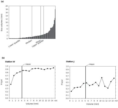
To accommodate the volume dependence, each position class was divided into two volume classes. To distinguish between small and large volumes, various limits were tested: mean, median, and upper and lower quartile of the box volumes in the position class. Figure 1a shows the typical location of these limits in an ordered plot of volumes. Since the lower quartile is located in a region of zero gradient and

the upper quartile is close to the mean, using quartiles was discarded. Comparative testing using mean and median, respectively, showed little difference in model parameters. Although using the median has the advantage of making the number of values in both volume classes equal, the mean was chosen as it is located approximately where the gradient starts to increase. This approach is also justified by the observed form of the increase of P(x/x) with increasing rainfall volume of the box to be branched. For both the Brazilian and British stations, the mean roughly localises the volume where P(x/x) approaches a plateau, although this is less pronounced in the Brazilian case where P(x/x) exhibits a larger scatter at higher volumes (Fig. 1b).

It has to be emphasised that the present cascade approach does not cover the correct reproduction of regularities in the timing of rainfall events at scales smaller than the one from which the disaggregation started. Thus, the diurnal patterns found for the Brazilian data (see Rainfall data section) cannot be reproduced. If such patterns are of practical relevance for further application of the disaggregated time series, the present model should not be used. Improving performance in this respect would require additional model parameters characterising the deterministic patterns, e.g. corresponding to the parameter storm starting time used in some previous approaches (e.g. Hershenhorn and Woolhiser, 1987).

Concerning model calibration, in the present study the original procedure of Olsson (1998) is modified in a number of ways. The main change is a weighting of the model parameters. For the P values this implies that, when averaging over a range of resolutions, each P value is assigned a weight according to the number of boxes used in its calculation. Generally, the higher the resolution, the larger the number of contributing boxes and consequently the higher the accuracy of the estimated P values. Another modification concerns the distribution of W_x/x. In Olsson (1998) both weights W₁ and W₂ were included, leading to symmetrical distributions (since W₁=1-W₂). While facilitating the fitting of a theoretical distribution, this means that any asymmetry in the empirical distribution of W₁ and

reflected in the distribution of the W₁ of isolated boxes. Thus, only the W₁ values are used to define the distribution of

W_x/x in the following analysis. This in turn means that a uniform distribution will not be a valid approximation. In fact, due to the strong variation in the shape of the empirical distribution between position and, to some extent, volume classes, fitting theoretical distributions is virtually impossible. Therefore, in the present study the actual empirical distributions are used in the disaggregation model. Based on the mean number of histogram values, the distributions are specified as seven-interval histograms. In the histograms, W₁ values from all resolutions within the studied range are pooled. This corresponds to the weighting of the P values, making the more accurately determined higher-resolution histograms exert greater influence.

The present studies focus exclusively on disaggregation

of daily values. Since the data employed are of a 1-hour resolution and since the cascade model implies resolutions expressed as the highest resolution multiplied by a power of two, the actual range used in the calibration is 1 (20_{) to}

32 (25_{) hours. To quantify the variation of the P values and}

the W_x/x histograms within this range, mean absolute differences were used. For each class and branching type, the differences were calculated between the weighted average P and the P of each resolution. Similarly, for each class and histogram interval, the differences were calculated between the pooled probability mass and the mass of each resolution (in this calculation three-interval histograms were used to decrease the statistical scatter).

For the British data, to assess intra-annual parameter variations, model calibration was carried out for each station’s total period and for seasonal subsets (winter:

Dec-Station W

Volume (mm)

0 1 2 3 4 5 6 7 8 9 10 11 12 13 14 15

P(x/x)

0.0 0.1 0.2 0.3 0.4 0.5 0.6 0.7 0.8 0.9

1.0 mean

Station J

Volume (mm)

0 1 2 3 4 5 6 7 8 9 10 11 12 13 14 15

P(x/x)

0.0 0.1 0.2 0.3 0.4 0.5 0.6 0.7 0.8 0.9 1.0

mean

>14 >14

Lower quartile

Median Mean Upper quartile

Box volumes (mm)

0 2 4 6 8 10 12 14 16 18 20

(a)

(b)

Fig. 1.(a) Typical location of mean and quantiles in an ordered plot of individual rainfall volumes belonging to a particular position class. (b)

Feb, spring: Mar-May, summer: Jun-Aug, autumn: Sep-Nov). For the Brazilian data, no seasonal subdivision was made since the amount of rainfall outside the Brazilian rainy season is very small and a separate parameter assessment for the dry period would be highly unreliable. Therefore, the parameter values are determined on the basis of the entire annual time series.

Following the model calibration, a range of disaggregation experiments was performed. When using the model for disaggregation, the class of each wet box is determined first, after which a random number is drawn to determine the type of branching. In the case of x/x, a second random number is drawn to determine W₁ and W₂. The experiments were separated into two parts, one termed theoretical and one termed practical. In the theoretical part, the total 1-hour time series for each station and season was aggregated into 32-hour values which were then disaggregated back to 1-hour values using the cascade model calibrated on the very same series (experiment E32/1). This is theoretical in the sense that, in practice, (1) the calibration data differ from the actual data to be disaggregated and (2), 32-hour values are never available. However, this type of experiment determines first of all whether the methodology is at all suited for disaggregation, and further provides the most accurate basis for comparing performance between stations and seasons.

The practical part corresponds to real-world model applications. In this respect, a critical issue is the discrepancy between the repeated resolution doubling inherent to the present, discrete cascade model and the frequent need to disaggregate (the commonly available) daily rainfall values into the hourly resolution commonly used in hydrological modelling. This limitation may be overcome by using a continuous cascade model, not based on resolution doubling but applicable between arbitrary scales (e.g. Tessier et al., 1993). The implementation of such models is, however, far more intricate and practicable schemes have yet to be developed and tested. Further, even if 1.5-hour or 45-min values (which can be directly ‘cascaded’ from daily values) could be accepted in the application, it is highly likely that the cascade model would have to be calibrated on hourly values since this is often the highest available time resolution of rainfall data. Two experiments were conducted to investigate how to overcome this discrepancy, both starting by aggregating the 1-hour volumes into daily values. In the first experiment (termed E24/32/1), the daily values were converted into a 32-hour resolution, firstly by dividing them into three equal 8-hour volumes and, secondly by aggregating the latter four by four. As an example, consider the series of daily values 0, 12, 0, 30 which is divided into the 8-hour volumes 0, 0, 0, 4, 4, 4, 0, 0, 0, 10, 10, 10 and

then aggregated to the 32-hour volumes 4, 8, 30. These ‘artificial’ 32-hour volumes were then disaggregated to 1-hour volumes with the cascade model. In the second experiment (termed E24/0.75/1), the daily values were directly disaggregated in five steps to 45-min volumes, which were then converted to 1-hour volumes in a similar fashion. Finally, the theoretical experiments were modified to consider two real-world scenarios. The first concerned infilling, i.e. to fill gaps in hourly series by disaggregating daily values from the same station using the model calibrated on existing hourly data. For this purpose, split-sample experiments (termed ESP32/1) were performed for each station in which the model was calibrated on two-thirds of the series and then used to disaggregate the remaining one-third. The second real-world scenario concerned spatial parameter transferability. This was tested by disaggregating the total period of each station using the parameters (i.e. P values and W_x/x distributions) of the other stations (experiment ETR32/1).

In each disaggregation experiment, 100 statistical realisations were generated and compared to observed 1-hour data in terms of four validation variables: individual 1-hour volume (iv), event volume (ev), event duration (ed), and length of the dry period between consecutive events (dp). Observed and generated data were compared in terms of mean and standard deviation of these variables. Moreover, extreme values were assessed by comparing both the absolute maximum value and the number of exceedances of thresholds specified as five and ten times the mean observed 1-hour volume of the actual period and station, Mn(iv).

the British values and, therefore, a minimum separation of four dry hours was chosen as the second event definition.

Besides mean and standard deviation, for each validation variable a root mean square relative error (MRE) was used to compare the entire distributions. From the data generated, an averaged list was constructed with the values in decreasing order for each realisation and then the first, second, etc. value of all realisations were averaged. This ordered list was compared with the observed ordered list by dividing the latter into bins of size 0.6 standard deviations of the actual variable, calculating the averages obs_i within each bin, and calculating the corresponding averages cal_i of the generated list. The binning was required to keep the

MRE value from being dominated entirely by the numerous

small values in the generally strongly skewed distributions; 0.6 standard deviations is a recommended bin size (Maniak, 1993). MRE of each validation variable was calculated as

(2)

and to obtain an overall measure of the accuracy of a certain disaggregation experiment, MRE was averaged over all seven variables (Mn(MRE)).

Results and discussion

CALIBRATION

Branching type probabilities P

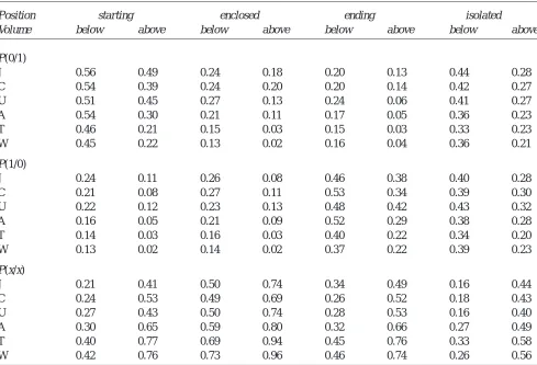
Empirical branching type probabilities P for each position and volume class and each station are presented in Table 2. A dependence of the probabilities on the box characteristics (i.e. rainfall volume and position in the rainfall sequence) was apparent for all stations. P(x/x) was higher for boxes above the mean volume than below mean volume (see also Fig.1b) and, further, was highest for enclosed boxes and lowest for isolated boxes. Due to two types of symmetries in the P values, the number of independent values may be reduced from 16 to 8. (1) P(0/1) for starting boxes is nearly identical to P(1/0) for ending boxes, and vice versa for starting boxes. (2) For enclosed and isolated boxes,

MRE cal obs

obs

i i

i

=  −



 

 

2

Table 2. Weighted probabilities P of the three types of division for all position and volume classes, derived from the total

observation period of each station, resolutions 1-32 hours.

Position starting enclosed ending isolated

Volume below above below above below above below above

P(0/1)

J 0.56 0.49 0.24 0.18 0.20 0.13 0.44 0.28

C 0.54 0.39 0.24 0.20 0.20 0.14 0.42 0.27

U 0.51 0.45 0.27 0.13 0.24 0.06 0.41 0.27

A 0.54 0.30 0.21 0.11 0.17 0.05 0.36 0.23

T 0.46 0.21 0.15 0.03 0.15 0.03 0.33 0.23

W 0.45 0.22 0.13 0.02 0.16 0.04 0.36 0.21

P(1/0)

J 0.24 0.11 0.26 0.08 0.46 0.38 0.40 0.28

C 0.21 0.08 0.27 0.11 0.53 0.34 0.39 0.30

U 0.22 0.12 0.23 0.13 0.48 0.42 0.43 0.32

A 0.16 0.05 0.21 0.09 0.52 0.29 0.38 0.28

T 0.14 0.03 0.16 0.03 0.40 0.22 0.34 0.20

W 0.13 0.02 0.14 0.02 0.37 0.22 0.39 0.23

P(x/x)

J 0.21 0.41 0.50 0.74 0.34 0.49 0.16 0.44

C 0.24 0.53 0.49 0.69 0.26 0.52 0.18 0.43

U 0.27 0.43 0.50 0.74 0.28 0.53 0.16 0.40

A 0.30 0.65 0.59 0.80 0.32 0.66 0.27 0.49

T 0.40 0.77 0.69 0.94 0.45 0.76 0.33 0.58

P(0/1)≈P(1/0). These findings agree with the results of

Olsson (1998) for Swedish rainfall time series and corroborate the relevance of a distinction into different box types.

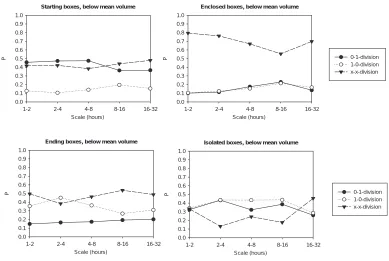
A measure of variation within the calibration range of 1 to 32 hours, the mean absolute differences between the weighted average P of Table 2 and P of each time resolution, was calculated to be 0.04–0.06 for the British stations and 0.06–0.08 for the Brazilian stations. The higher variation of the Brazilian stations can be attributed mainly to a larger statistical scatter between scales due to the lower number of rainy intervals in the Brazilian data (Table 1). When determining P values for a shortened British time series with the same number of rainy intervals as in the Brazilian case, the resulting variation of P with time scale was even larger than that for the semi-arid climate. Looking at P values as a function of time scale, no trends could be recognised in most cases. An exception might be the slight increase of P(x/x) with increasing time resolution for enclosed boxes (Fig. 2 for station W). A similar pattern was found for the other stations. Thus, scale invariance of P in the range of 1 hour to 32 hours was considered to be a reasonable assumption in this study. This is in line with the results of Olsson (1998) who found that P values were fairly constant for time scales above 1 hour.

Mean differences of P values between seasonal subsets were generally small for all British stations (0.03, 0.07 and 0.04 for stations A, T and W) and did not expose any obvious pattern when comparing spring, autumn and winter. For the summer, however, P(x/x) was lower than in any other season, particularly when compared to winter. This observation is due to a more frequent occurrence of convective rainfall events in the temperate climate during the summer. Their shorter event duration leads to a higher probability of rainfall occurring in only one of two successive time intervals, i.e. a lower P(x/x).

For the British stations, mean absolute differences in P values of the total time series were small when comparing stations T and W, but considerably higher between stations A and T or A and W, respectively (Table 3a). In fact, the pattern of P values between position and volume classes was identical for stations W and T, whereas P(x/x) for station A was on average 0.1 lower than P(x/x) of W and T (Table 2 and Table 3b). This reflects the location of A within the temperate climate, characterised by a higher probability of convective events. Differences in P between the Brazilian stations were similar to the homogeneous British stations W and T (Table 3a). These differences, however, could not be attributed to any systematic deviation of P between branching types or position/volume classes (Table 2). They Starting boxes, below mean volume

Scale (hours)

1-2 2-4 4-8 8-16 16-32

P

0.0 0.1 0.2 0.3 0.4 0.5 0.6 0.7 0.8 0.9 1.0

0-1-division 1-0-division x-x-division Enclosed boxes, below mean volume

Scale (hours)

1-2 2-4 4-8 8-16 16-32

P

0.0 0.1 0.2 0.3 0.4 0.5 0.6 0.7 0.8 0.9 1.0

Ending boxes, below mean volume

Scale (hours)

1-2 2-4 4-8 8-16 16-32

P

0.0 0.1 0.2 0.3 0.4 0.5 0.6 0.7 0.8 0.9 1.0

0-1-division 1-0-division x-x-division Isolated boxes, below mean volume

Scale (hours)

1-2 2-4 4-8 8-16 16-32

P

0.0 0.1 0.2 0.3 0.4 0.5 0.6 0.7 0.8 0.9 1.0

Fig. 2. Empirical probabilities P(0/1), P(1/0) and P(x/x) as function of time scale for all position classes below mean volume, station W

may be associated with larger uncertainties in the case of the Brazilian data, where the number of elements is small, in particular for the above-mean volume classes.

Differences in P values between the two climates were large, with the British station A being closer to the Brazilian characteristics than T and W (Table 3a). The main feature which distinguishes probabilities of the semi-arid climate from those of the temperate climate refers to P(x/x), which is substantially lower in the semi-arid for all position and volume classes (Table 2 and Table 3b). Furthermore, differences in the P(0/1) and P(1/0) values for starting and ending boxes were more pronounced in the British data (Table 2). The reason for both these observations is the dominance of short-term convective rainfall events in the tropical climate which implies a lower probability of long-duration rainfall sequences than advective events. The latter comprise a continuous sequence of wet intervals also at a higher time resolution thus producing larger P(x/x) values. Concerning starting and ending boxes, the probability of having, for example, a 0/1-division for a starting box is thus higher than in the semi-arid case. There it is more probable that this box belongs to an independent short-term rainfall event at a higher time resolution, resulting in a 1/0-division at some cascade level. This reasoning is similar to that applied for seasonal differences in the temperate climate, although leading there to a considerably smaller effect in terms of a decreasing P(x/x) in summer.

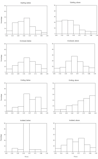
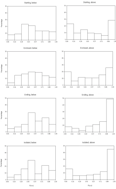
Distribution of W_x/x

Figures 3 and 4 show typical examples of pooled W_x/x histograms for all position and volume classes in both climates. For the class below mean rainfall volume, the histograms exhibit an approximately triangular distribution with its peak around 0.5. The triangular shape was less pronounced for the Brazilian data, particularly when comparing the position class of isolated boxes which was almost completely dominated by the 0.5 histogram class in

the British data. This implies that it is more likely for a certain rainfall volume to be composed of evenly distributed volumes at a higher time resolution in the temperate climate than in the semi-arid climate. Principal rainfall characteristics of both climates are thus reflected properly. Temperate-climate rainfall events are characterised by a long duration with intensities remaining roughly constant during subsequent intervals while the tropical climate is characterised by short-term events with highly time-variable intensities. The histograms of starting and ending boxes of the British stations are characterised by a skewness in shape, with W_x/x<0.5 being more frequent than W_x/x>0.5 for starting boxes and vice versa for ending boxes. This is physically reasonable as for starting boxes a larger share of the rainfall volume is attributed to the second half, thus closer in time to the centre of the rainfall event. This tendency was even more pronounced with increasing rainfall volume (moving from the below-mean to the above-mean volume class), making the approximately triangular distribution having its maximum at the smallest (largest) W_x/x values for the starting (ending) class. These observations justify the use of asymmetrical histograms for W_x/x, as internal event asymmetries do indeed exist in the analysed data and can consequently be reflected in the disaggregation procedure. For the Brazilian data, the triangular distributions of W_x/x in the below-mean volume classes inverted into an approximately V-shape for all above-mean volume classes. It is thus more likely for large rainfall volumes to be separated into two uneven parts than for smaller volumes, even for enclosed and isolated boxes. In the below-volume class, the maximum possible W_x/x is defined by the ratio of the mean volume to the maximum resolution of the measurement device. In the above-volume class, ratios can be considerably higher, thus resulting in broader distributions of W_x/x which automatically puts stronger weight on the marginal histogram classes.

In testing the scale-invariance of the histograms for the range of time scales under consideration, a visual inspection

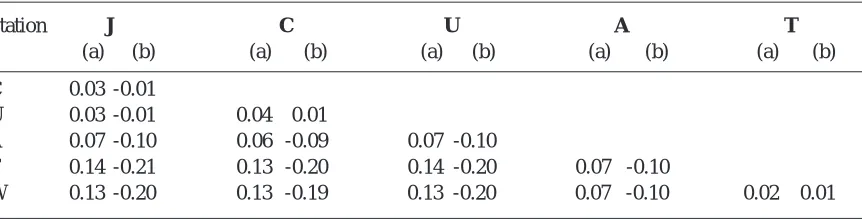
Table 3. Mean absolute difference of all P values between all stations, averaged over all position and volume

classes and all branching types (a). Mean difference of P(x/x) between all stations, averaged over all position and volume classes (b).

Station J C U A T

(a) (b) (a) (b) (a) (b) (a) (b) (a) (b)

C 0.03 -0.01

U 0.03 -0.01 0.04 0.01

A 0.07 -0.10 0.06 -0.09 0.07 -0.10

T 0.14 -0.21 0.13 -0.20 0.14 -0.20 0.07 -0.10

Starting, below

0.00 0.14 0.29 0.43 0.57 0.71 0.86 1.00

Percentage

0 10 20 30 40 50

Enclosed, below

0.00 0.14 0.29 0.43 0.57 0.71 0.86 1.00

Percentage

0 10 20 30 40 50

Ending, below

0.00 0.14 0.29 0.43 0.57 0.71 0.86 1.00

Percentage

0 10 20 30 40 50

Isolated, below

P(x-x)

0.00 0.14 0.29 0.43 0.57 0.71 0.86 1.00

Percentage

0 10 20 30 40 50

Starting, above

0.00 0.14 0.29 0.43 0.57 0.71 0.86 1.00 0

10 20 30 40 50

Enclosed, above

0.00 0.14 0.29 0.43 0.57 0.71 0.86 1.00 0

10 20 30 40 50

Ending, above

0.00 0.14 0.29 0.43 0.57 0.71 0.86 1.00 0

10 20 30 40 50

Isolated, above

P(x-x)

0.00 0.14 0.29 0.43 0.57 0.71 0.86 1.00 0

10 20 30 40 50

Starting, below

0.00 0.14 0.29 0.43 0.57 0.71 0.86 1.00

Percentage

0 10 20 30 40 50

Enclosed, below

0.00 0.14 0.29 0.43 0.57 0.71 0.86 1.00

Percentage

0 10 20 30 40 50

Ending, below

0.00 0.14 0.29 0.43 0.57 0.71 0.86 1.00

Percentage

0 10 20 30 40 50

Isolated, below

P(x-x)

0.00 0.14 0.29 0.43 0.57 0.71 0.86 1.00

Percentage

0 10 20 30 40 50

Starting, above

0.00 0.14 0.29 0.43 0.57 0.71 0.86 1.00 0

10 20 30 40 50

Enclosed, above

0.00 0.14 0.29 0.43 0.57 0.71 0.86 1.00 0

10 20 30 40 50

Ending, above

0.00 0.14 0.29 0.43 0.57 0.71 0.86 1.00 0

10 20 30 40 50

Isolated, above

P(x-x)

0.00 0.14 0.29 0.43 0.57 0.71 0.86 1.00 0

10 20 30 40 50

of histograms for different resolutions revealed a generally large scatter, particularly for classes with a small number of values. For the same reason, the variation was larger for the three Brazilian stations, where mean absolute interval differences were in the range of 9.0–11.8, compared to a range of 7.3–8.3 for the British stations. Nevertheless, the general pattern of histogram shapes discussed above could in principle be observed for all time scales in the range of 1–32 hours. However, a clear trend was present for enclosed boxes, whose histogram shape changes from triangular at small time scales to approximately uniform, or even V-shaped for the semi-arid case, at larger time scales. Thus, the probability of one rainfall volume being divided into two uneven volumes decreases with increasing resolution in favour of a smoother separation. However, as this tendency was not obvious for other position classes and less significant for the Brazilian data than for the British, the scale-invariance of W_x/x distributions in the scaling range of this study was considered to be fulfilled.

DISAGGREGATION

Theoretical experiments

Results of disaggregation experiments E32/1 are given in Table 4 (part I). For all stations, the number of non-zero 1-hour intervals and their mean rainfall volume were reproduced accurately by the model. The standard deviation of individual volumes was slightly overestimated, pointing to intervals with too high generated rainfall volumes. Assessing the performance of disaggregations in the view of event characteristics, and taking one dry hour as a minimum interval between two events, Table 4 shows that event durations were underestimated by the model for all stations. The number of generated events was too high, although the number of individual volumes was represented adequately. This indicates that continuous sequences of wet boxes were split up too frequently into separate events. Consequently, event volumes and the length of dry periods were underestimated. The overall distribution of dry periods, however, was well represented (MRE(dp₁) in Table 4) mainly because long dry periods are preserved by the model during disaggregation. In terms of the second event definition (four dry hours as minimum separation between events), the performance of the cascade model is very satisfactory. Mean and standard deviation of event volumes, event duration and length of dry periods were generated accurately, the difference in performance between climates is low. Summarising disaggregation results for all validation variables (Mn(MRE) in Table 4), the stations in the semi-arid climate, dominated by convective rainfall events,

perform better than the stations in the temperate climate. Variation in performance between the stations in the semi-arid climate is low. Variations within the temperate climate are more pronounced, related mainly to the overestimation of extreme values of individual rainfall volumes. Performance improves with decreasing annual rainfall and increasing influence of convection on rainfall generation.

Typical autocorrelation functions for both climates (Fig. 5) were generally considerably underestimated by the model. In the semi-arid climate, autocorrelation is lower than in the temperate climate due to the short-duration rainfall events. Nevertheless, an increase of correlation for shorter time lags was, in principle, reproduced by the model. This may be attributed to the model taking into account specific parameters for different position classes and unsymmetrical distributions of W_x/x which both enable representation, to some extent, of the correlation structures between successive intervals.

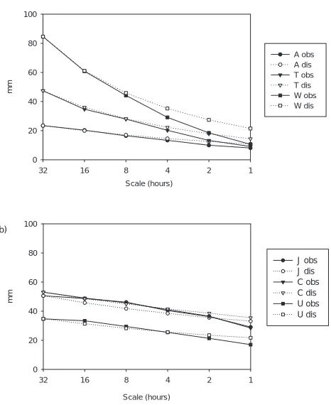
Concerning extreme values (Table 5), an overestimation was observed in particular for the British stations. Too many volumes exceeding the five times mean volume threshold were generated for stations W and T, whereas the number was well reproduced for the other stations. For the higher threshold (ten times the mean volume), an overestimation appeared for all stations, more severe for the British than for the Brazilian stations. Accordingly, the MRE of individual volumes deteriorated in the same way. For an explanation of these differences in model performance between the stations, consider the ensemble of the 20 largest interval volumes at different time scales (Table 5 and Fig. 6). As expected, mean maximum volumes decrease with increasing time resolution, although for the semi-arid climate the decrease is considerably lower than for the temperate, in particular compared to station W. This is reasonable in the view of the dominating rainfall mechanisms. Rainfall events of long duration at the British stations accumulate to large volumes at a lower time resolution, whereas for the Brazilian stations large volumes are composed mainly of singular short events with high intensities. The cascade model, however, was not able to represent the decrease of extreme volumes adequately in cases where the ratio between mean maximum 32- and 1-hour volumes was high in the original data, i.e. in the temperate climate with high annual rainfall.

Station J C U

obs I II obs I II obs I II

(a)

No(iv) 1253 1258 1504 1205 1206 1449 634 616 708 Mn(iv) 2.7 2.7 2.2 2.7 2.7 2.3 2.1 2.2 1.9 Sd(iv) 5.2 5.3 4.6 5.1 5.7 4.7 3.7 4.6 4.0

MRE(iv) 0.13 0.13 0.19 0.14 0.30 0.25

No(ev₁) 668 802 728 622 755 689 339 410 361 Mn(ev₁) 5.0 4.2 4.6 5.3 4.4 4.8 4.0 3.3 3.7 Sd(ev₁) 10.1 7.7 8.8 10.7 8.4 9.2 9.1 6.8 7.9 MRE(ev₁) 0.21 0.14 0.21 0.14 0.21 0.11 Mn(ed₁) 1.9 1.6 2.1 1.9 1.6 2.1 1.9 1.5 2.0 Sd(ed₁) 1.6 1.0 1.4 1.7 1.1 1.5 1.8 1.0 1.4 MRE(ed₁) 0.26 0.16 0.26 0.15 0.32 0.19 Mn(dp₁) 46.7 38.9 42.5 52.6 43.4 47.1 64.0 53.0 59.8 Sd(dp₁) 183.8 168.4 176.1 152.8 140.3 145.5 155.9 143.2 152.1 MRE(dp₁) 0.01 0.01 0.01 0.02 0.01 0.01 No(ev₄) 519 518 504 486 494 482 261 277 263 Mn(ev₄) 6.4 6.4 6.6 6.8 6.7 6.8 5.2 4.9 5.1 Sd(ev₄) 11.7 10.8 11.4 12.1 11.5 12.0 10.6 9.6 10.2 MRE(ev₄) 0.09 0.05 0.07 0.04 0.10 0.06 Mn(ed₄) 2.9 3.4 3.8 3.0 3.3 3.8 2.9 3.0 3.3 Sd(ed₄) 3.7 3.8 3.9 2.9 3.7 3.9 3.1 3.5 3.5 MRE(ed₄) 0.25 0.30 0.27 0.35 0.14 0.17 Mn(dp₄) 59.7 59.3 60.5 66.9 65.3 66.5 82.6 77.4 81.9 Sd(dp₄) 206.7 206.8 209.1 170.2 169.5 170.3 173.5 168.7 173.8 MRE(dp₄) 0.01 0.01 0.01 0.01 0.01 0.01

Mn(MRE) 0.14 0.11 0.15 0.12 0.15 0.12

(b)

No(iv) 2760 2828 3105 7299 7195 7790 7709 7740 8376 Mn(iv) 0.85 0.83 0.76 0.92 0.93 0.86 1.3 1.3 1.2 Sd(iv) 1.1 1.3 1.1 1.1 1.3 1.2 1.6 1.9 1.7

MRE(iv) 0.35 0.16 0.44 0.31 0.71 0.55

No(ev₁) 1126 1482 1305 2216 2785 2479 2043 2661 2324 Mn(ev₁) 2.1 1.6 1.8 3.0 2.4 2.7 4.9 3.8 4.3 Sd(ev₁) 3.7 2.6 2.9 6.5 4.4 5.2 11.4 7.7 9.0 MRE(ev₁) 0.23 0.20 0.29 0.20 0.29 0.20 Mn(ed₁) 2.5 1.9 2.4 3.3 2.6 3.1 3.8 2.9 3.6 Sd(ed₁) 2.5 1.4 1.9 4.1 2.5 3.2 4.7 3.0 4.0 MRE(ed₁) 0.33 0.23 0.34 0.21 0.28 0.14 Mn(dp₁) 32.8 24.8 28.0 12.5 10.0 11.0 12.8 9.8 11.0 Sd(dp₁) 64.7 57.7 61.0 24.7 22.0 23.4 26.6 24.0 25.5 MRE(dp₁) 0.02 0.02 0.05 0.05 0.04 0.04 No(ev₄) 748 836 797 1113 1227 1203 1073 1109 1089 Mn(ev₄) 3.1 2.8 3.0 6.0 5.5 5.6 9.3 9.0 9.2 Sd(ev₄) 4.8 4.3 4.4 10.5 10.0 8.1 18.9 17.7 18.1 MRE(ev₄) 0.09 0.07 0.08 0.04 0.12 0.11 Mn(ed₄) 4.5 4.7 5.0 8.1 7.8 8.2 8.6 9.2 9.5 Sd(ed₄) 4.7 5.1 5.3 9.6 9.9 10.3 11.2 11.8 12.3 MRE(ed₄) 0.15 0.18 0.13 0.16 0.09 0.12 Mn(dp₄) 48.5 42.8 44.8 23.3 20.7 20.9 23.0 21.4 21.6 Sd(dp₄) 74.6 71.9 73.3 31.3 29.9 30.6 33.7 33.9 34.2 MRE(dp₄) 0.03 0.02 0.05 0.05 0.05 0.05

Mn(MRE) 0.17 0.13 0.19 0.15 0.27 0.17

Table 4. Comparison between observed (obs) and disaggregated 1-hour time series for Brazilian stations

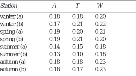
no significant effect on the quality of disaggregation results. This applies even for the summer season, where parameter variation relative to the remaining seasons was most pronounced. An improvement with respect to the number of generated rainy intervals was counteracted by a decrease in the performance of extreme value simulations, leading to a similar or even higher Mn(MRE) using seasonal parameters. This suggests that the intra-annual parameter variations may be neglected in view of overall model performance in the temperate climate. However, disaggregation accuracy is highest during summer (Table 6), in line with the previously observed model improvement with increasing influence of convective rainfall generation.

Practical experiments

Experiments E24/32/1 and E24/0.75/1 compare two approaches for disaggregation of daily to hourly time series which deal with the restriction to specific time resolutions inherent in the cascade model. Results were considerably

Lag (hour)

1 2 3 4 5 6 7 8 9 10

Correlation

0.0 0.2 0.4 0.6 0.8

C obs C E32/1 C E24/0.75/1 T obs T E32/1 T E24/0.75/1

Fig. 5. Autocorrelation for observed and disaggregated

(experi-ments E32/1 and E24/0.75/1) 1-hour time series for stations C (semi-arid climate) and T (temperate climate).

Table 5: Performance of disaggregated versus observed 1-hour data with regard to extreme rainfall volumes

for each station, experiment E32/1. (iv: 1-hour rainfall volume [mm], Mn: mean, Max: maximum, NE: number of exceedances, nMn: volume threshold of n times Mn(iv), LT: the 20 largest rainfall volumes at the T-hour level.)

Station J C U A T W

obs dis obs dis obs dis obs dis obs dis obs dis

Mn(iv) 2.7 2.7 2.7 2.7 2.1 2.2 0.85 0.83 0.92 0.93 1.3 1.3

Max(iv) 60.2 60.9 48.4 65.3 25.2 53.4 12.6 23.2 15.0 26.9 12.6 43.0

NE(5Mn) 56 50 59 50 26 22 59 60 147 160 140 166

NE(10Mn) 9 13 7 13 5 7 4 13 5 28 0 32

MRE(iv) 0.13 0.19 0.30 0.35 0.44 0.71

Mn(L32) 50.6 50.6 53.0 53.0 34.7 34.7 23.4 23.4 47.4 47.4 84.6 84.6

Mn(L1) 29.1 33.1 28.4 35.5 17.0 21.7 8.1 10.8 9.1 14.3 10.6 21.5

Mn(L32)/ Mn(L1) 1.7 1.5 1.9 1.5 2.0 1.6 2.9 2.2 5.2 3.3 8.0 3.9

a)

Scale (hours)

32 16 8 4 2 1

mm

0 20 40 60 80 100

A obs A dis T obs T dis W obs W dis

b)

Scale (hours)

32 16 8 4 2 1

mm

0 20 40 60 80 100

J obs J dis C obs C dis U obs U dis

Fig 6. Mean of the 20 largest interval volumes as function of time scale, observed (obs) and disaggregated (dis, experiment E32/1)

better for E24/0.75/1. The principal problem of E24/32/1 is a large overestimation of the number of rainy intervals (No(iv)) which makes all other validation variables perform unsatisfactorily, too. For E24/0.75/1, there was also an overestimation of No(iv) of about 17% for the Brazilian stations and 9% for the British stations. However, this was considerably lower than for E24/32/1 and the results in terms of all other validation variables were also superior for E24/ 0.75/1. It is concluded that the conversion of 45-min values to 1-hour values after disaggregation is preferable to the conversion of 24-hour values to 32-hour values before disaggregation. The reason is that the percentage of rainy intervals is higher in the converted data series than in the original ones. Therefore, No(iv) is overestimated in both experiments, but to a considerably larger extent in E24/32/1 because the error is increased at each disaggregation step. In fact E24/0.75/1 in most respects performed better than not only E24/32/1 but also (the theoretical) E32/1 (Table 4). This indicates that the higher level of detail in the 24-hour values is important and that disaggregation generally should start from as high a resolution as possible. However, the conversion from 45 min to 1 hour may also have influenced the results positively. Figure 7 compares the distributions of validation variables in observed 1-hour values and 1-hour values disaggregated in E24/0.75/1. The overall agreement was generally good, in particular for the Brazilian stations, with some deviations of the disaggregated time series occurring in the reproduction of extremes. One-hour volumes were overestimated for the British stations, whereas event duration and volume (for minimum event separation of 1 dry hour) were somewhat underestimated in both climates. Event characteristics for the definition of 4 dry hours as minimum separation between events were generally better represented.

The slight overestimation of event duration in this case is an effect of the excessive number of non-0 intervals (Table 4, part II), which split up dry periods, thereby concatenating two rainfall sequences into one event. The overestimation of No(iv) was larger for the semi-arid data. This is due to their lower percentage of rainy intervals, which implies that the impact of the artificial increase of No(iv) resulting from data conversion is relatively more apparent. For both climates, the complete distributions of individual 1-hour volumes were represented even better than in the theoretical disaggregations of real 32-hour time series, E32/1 (Table 4). The main reason is a reduced overestimation of extreme volumes, which can be attributed at least partly to the smoothing of intensities while converting from 45-min to 1-hour values. Autocorrelation functions for both climates were better represented in E24/0.75/1 than in E32/1 with a particular improvement at lag 1 hour (Fig. 5). This is also partly related to the conversion approach, where the rainfall volume of one disaggregated 45-min interval may be distributed to two 1-hour intervals, thereby increasing the correlation between successive intervals. Other differences in performance between stations and climates are similar in their structure to those discussed in the section on theoretical experiments.

The results from experiment E24/0.75/1 may be compared with the results from previous approaches to rainfall disaggregation in the same scale range. For methods based on distribution-fitting of event characteristics, performance is generally evaluated in terms of ev and ed. Hershenhorn and Woolhiser (1987) used the two-sample Kolmogorov-Smirnov test to verify the hypothesis that observed and simulated distributions of ev and ed were statistically similar (significance level 0.05). For the binned values of ev and

ed used to calculate MRE, this hypothesis could not be

rejected for any of the stations in the present study. Connolly

et al. (1998) used a parameter EF, essentially measuring

the closeness to the line x=y in plots such as Fig.7 and, for their stations, found on average EF≈0.8 for both ev and ed when excluding the 5% highest values (EF=1 means perfect match). For the present data, the equivalent EF values are generally >0.95 for the plots in Fig.7, somewhat lower (~0.7) for ed, station J. For disaggregation methods based on rectangular pulses models, performance has been evaluated in terms of the 1-hour structure by the fraction of zero-values (f(0)), variance (Va), and lag-1 autocorrelation (Acf(1)). Very generally, the models have reached a near-perfect f(0), Acf(1) within 10% of observed value, and Va within 20% of observed value (e.g. Bo et al., 1994; Glasbey et al., 1995). The accuracy of simulations are of similar quality, somewhat lower for Acf(1) and higher for Va. Overall the performance of the present model compares favourably with previous

Table 6. Performance of disaggregation of seasonal subsets

in terms of Mn(MRE) with seasonal parameters (a) and total parameters (b), stations A, T and W (temperate climate). (winter: Dec-Feb; spring: Mar-May; summer: Jun-Aug; autumn: Sep-Nov).

Station A T W

winter (a) 0.18 0.18 0.20

winter (b) 0.17 0.21 0.22

spring (a) 0.19 0.20 0.21

spring (b) 0.19 0.21 0.20

summer (a) 0.14 0.15 0.18

summer (b) 0.13 0.10 0.18

autumn (a) 0.18 0.18 0.23

iv

obs (mm)

0 5 10 15 20 25 30

dis (mm)

0 5 10 15 20 25 30

ev1

obs (mm)

0 20 40 60 80 100

dis (mm)

0 20 40 60 80 100

ed1

obs (hours)

0 10 20 30 40 50 60

dis (hours)

0 10 20 30 40 50 60

dp1

obs (hours)

0 100 200 300 400

dis (hours)

0 100 200 300 400

ev4

obs (mm)

0 20 40 60 80 100

dis (mm)

0 20 40 60 80 100

ed4

obs (hours)

0 20 40 60 80 100

dis (hours)

0 20 40 60 80 100

iv

obs (mm)

0 20 40 60 80

dis (mm)

0 20 40 60 80

ev1

obs (mm)

0 20 40 60 80

dis (mm)

0 20 40 60 80

ed1

obs (hours)

0 5 10 15 20

dis (hours)

0 5 10 15 20

dp1

obs (hours)

0 1000 2000 3000

dis (hours)

0 1000 2000 3000

ev4

obs (mm)

0 20 40 60 80

dis (mm)

0 20 40 60 80

ed4

obs (hours)

0 10 20 30 40 50 60

dis (hours)

0 10 20 30 40 50 60

(b) (a)

Fig. 7. Comparison of distributions of validation variables for observed and disaggregated 1-hour data for (a) station T, temperate climate,

approaches.

Besides the practical relevance of extending high resolution rainfall time series of stations where only a short period of 1-hour measurements are available, split-sample tests are a more rigorous validation method, examining the transferability of model parameters (and concepts) in time. The results of the split-sample disaggregations exhibit a notable difference between the climates (Table 7). Whereas for the British stations the performance in terms of Mn(MRE) and the number of generated wet 1-hour boxes was equal to or even better than the disaggregations of the complete time series (Table 4), a decline in performance was observed for the Brazilian stations. Within the semi-arid climate, No(iv) was overestimated for stations J and C and severely underestimated for station U. The differences in parameters between the calibration and the validation period were considerably larger for the semi-arid than for the temperate data, both in terms of P values and W_x/x histograms (Table 7). The main feature of these differences was a markedly higher P(x/x) in the calibration period of stations J and C and the opposite for station U. This explains the observed deviations of generated No(iv) in the split-sample disaggregation. For the British stations, the differences in parameters were low and, consequently, performance of the split-sample test was comparable to the disaggregations of the complete data period. The improvement of Mn(MRE) for station W was due exclusively to a better representation of extreme values, which might be chance.

Two possible explanations for the higher variation of the semi-arid parameters exist. First, the number of rainy hours per year is roughly seven times lower for the semi-arid hourly data leading to a higher statistical scatter (Table 1). Second, the higher interannual variability of precipitation in the semi-arid study area implies that the parameter set calibrated on one year might not be adequately applicable

in the next year. Consequently, longer time series are needed to obtain a calibration quality similar to that of the temperate climate. The 1.5 year calibration period of station U is at the lower limit of a sound applicability for the present approach as the number of values in some classes is small. On the other hand, to get all properties of the cascade generator estimated accurately, a larger total number of rainy intervals is required in the temperate climate due to the dominance of the enclosed position class (Table 1). In the semi-arid climate, rainfall is more equally distributed among position classes, leading to a similar quality of parameter estimation.

Another objective of practical relevance was to test the spatial transferability of parameters. In Table 8, disaggregation performance is compared for all combinations of stations in both climates. The results reflect, closely, differences in parameters between station and climates. For the stations within the semi-arid climate, disaggregation results were very similar. Thus, the parameters of one station can be applied for disaggregation of another station without any remarkable loss in performance. The same applies for stations W and T in the temperate climate. The parameters of station A, characterised by considerably lower mean annual rainfall, could not be applied for stations W and T, however, without a pronounced loss in model performance. Notably, the model performance for station A was similar with parameters from all the other stations in terms of Mn(MRE), although with deviations in an opposite sense (see No(iv)) when applying the British or Brazilian parameters. The rainfall regime of station A has thus intermediate properties with respect to the parameterisation of the cascade model. This can be related to the general tendency for convective rainfall activity to play a greater role in the south and east of the British Isles than in the north and west. A detailed weather

Table 7. Comparison between observed (obs) and disaggregated 1-hour time series

for experiments ESP32/1 and E32/1. Diff(P): Mean differences of P values between calibration and validation period, averaged over all position and volume classes and all branching types, Diff(W_x/x): Mean difference of pooled histograms between calibration and validation period, averaged over all position and volume classes.

Station J C U A T W

No(iv), obs 401 401 261 1010 2615 2651

No(iv), ESP32/1 430 486 203 949 2570 2576

Mn(MRE), ESP32/1 0.15 0.18 0.19 0.17 0.18 0.23

Mn(MRE), E32/1 0.14 0.15 0.15 0.17 0.19 0.27

Diff(P) 0.04 0.05 0.07 0.03 0.04 0.04

type analysis of the specific rainfall time series used is not available. As expected, the model performance was poorest when the semi-arid parameters were applied to station W and T and vice versa.

Summary and conclusions

A temporal rainfall disaggregation model based on the principles of random multiplicative cascade processes was applied in two contrasting climates, a semi-arid tropical (Brazil) and a temperate (United Kingdom). The aim was to convert daily time series into an hourly resolution. In this range of time scales, the scale-invariant assumptions of the model were shown to be approximately equally well fulfilled for both climates. The model parameters differed distinctly reflecting the dominance of convective processes in the Brazilian rainfall and of frontal passages in the British rainfall. In the British case, the parameters exhibited a slight seasonal variation consistent with the higher frequency of convection during summer. When applied for disaggregation, the model reproduced a range of hourly rainfall characteristics with high accuracy in both climates. However, the overall model performance was somewhat better for the semi-arid tropical rainfall. In particular, extreme rainfall was constantly overestimated for the British stations whereas extreme rainfall in Brazil was well reproduced. Transferability of parameters in time was seen to be associated with larger uncertainty in the semi-arid climate due to its higher interannual variability and lower percentage of rainy intervals. For parameter transferability in space, no restrictions were found between the Brazilian stations whereas in the UK regional differences were more pronounced. Mean annual rainfall is a potentially appropriate measure to which parameter variations within the temperate

climate can be related.

The present study is, to the authors’ knowledge, the first to address differences in not only the parameters but also the performance of a cascade-based rainfall model with geographical region and governing rainfall processes. Concerning the parameters, their variation could be interpreted directly in terms of the physical processes involved. Concerning the performance, this improved with increasing rainfall variability, in turn associated with an increasing convective activity. The poorer performance for frontal-dominated temperate regions was manifested mainly in an overestimation of extreme rainfall, or more specifically in an inability of the model to reproduce a sharp decrease in maxima with increasing temporal resolution. For other cascade models, explicit extreme value analyses have generally not been performed. Thus, it is hard to conclude whether this is a general problem of cascade models or is specific to the present scheme. However, the necessity to smooth singularities as the cascade proceeds towards higher resolution when dealing with geophysical fields has been recognised previously (e.g. Marshak et al., 1994). This has prompted the development of so-called bounded cascades for rainfall, whose parameters depend explicitly on the actual resolution (e.g. Menabde et al., 1997, 1999). In the present framework, singularity smoothing would amount to having

P(x/x) and/or the fraction of probability mass located close

to the centre of the W_x/x histograms increasing with increasing resolution. Such tendencies are indeed present in the data sets but the increase is weak and did not appear sufficient to abandon the scale-invariant model assumptions which performed well for the semi-arid case. Alternative possible means of improving model performance with respect to extreme values in the temperate climate include incorporating a third volume class with specific parameters

Table 8. Performance of disaggregated 1-hour time series for all stations in terms of Mn(MRE) (a) and

No(iv) (b). Experiment ETR32/1. (bold: Performance of disaggregation of one station with parameters of the same station.)

Disaggregation of station:

J C U A T W

(a) (b) (a) (b) (a) (b) (a) (b) (a) (b) (a) (b)

with parameters of station:

J 0.14 1285 0.14 1166 0.16 612 0.27 1832 0.54 3256 0.66 3320

C 0.14 1293 0.15 1206 0.16 628 0.27 1896 0.53 3316 0.66 3352

U 0.14 1266 0.15 1175 0.15 616 0.26 1854 0.51 3274 0.63 3346

A 0.24 1860 0.24 1717 0.22 882 0.17 2828 0.35 5041 0.45 5100

T 0.47 2737 0.48 2513 0.40 1279 0.20 3865 0.19 7195 0.25 7404

for extreme values or defining the P values as functions of the rainfall volume. Representing rainfall from contrasting climates may require not only adjusting the parameters but also using a conceptually different cascade model framework.

Besides the extreme value overestimation for some stations, the overall high accuracy of model disaggregated data supports its potential usefulness in hydrological applications. Some open questions are related to the time scales of applicability. The present study was confined to the range 1 day to 1 hour but useful disaggregation may be possible to even smaller scales. Another workable experiment is to calibrate the model using only a daily time series and evaluate up to which resolution disaggregation of the same series can be performed accurately. This possibility is a notable advantage of the present model compared with existing alternatives. Finally, besides assessing the quality of disaggregated data solely by comparison with observations, tests using the disaggregated data in hydrological modelling are required to evaluate their practical value. Early tests of cascade-disaggregated rainfall from daily to hourly time intervals with a simple runoff modelling approach (Calver, 1996) suggest that, over periods of the length used in the testing above, water resource issues are likely to be covered adequately by cascaded rainfall. It is, however, in the modelling of floods, particularly the more extreme events, that synthetic rainfall may introduce error. This comment should, however, be set in the context that other sources contribute to error in flood frequency modelling, notably in model structure and parameter identifiability. Moreover, an accurate description of not only the temporal but also the spatial rainfall distribution is crucial for successful hydrological modelling. Assessing the potential of the cascade methodology in this respect is an important area of future research.

Acknowledgements

Funding for AG and for data capture in Brazil was provided from both the German Ministry for Education and Research (BMBF) and the Brazilian Conselho Nacional de Desenvolvimento Científico e Tecnológico (CNPq) within the co-operation programme WAVES. JO was funded by a European Commission S&T Fellowship jointly with the Japan Society for the Promotion of Science. AC and BG gratefully acknowledge funding from the England and Wales Ministry of Agriculture, Fisheries and Food. The reviewers are thanked for helpful and constructive criticism.

References

Barry, R.G. and Chorley, R., 1987. Atmosphere, Weather and Climate. Methuen, 5th edition.

Bo, Z., Islam, S. and Eltahir, E.A.B., 1994. Aggregation-disaggregation properties of a stochastic rainfall model. Water Resour. Res., 30, 3423–3435.

Buishand, T.A., 1977. Stochastic modeling of daily rainfall sequences. Mededelingen Landbouwhogeschool, Wageningen, Netherlands, 77–3.

Calver, A. 1996. Development and experience of the Tate rainfall-runoff model. Proc. Inst. Civil Engrs: Water, Maritime and Energy, 118, 168–176.

Connolly, R.D., Schirmer, J. and Dunn, P.K., 1998. A daily rainfall disaggregation model. Agric. Forest Meteorol., 92, 105–117. Cowpertwait, P.S.P., O’Connell, P.E., Metcalfe, A.V. and

Mawdsley, J.A., 1996. Stochastic point process modelling of rainfall. II. Regionalisation and disaggregation. J. Hydrol., 175, 47–65.

Deidda, R., Benzi, R. and Siccardi, F., 1999. Multifractal modeling of anomalous scaling laws in rainfall. Water Resour. Res., 35, 1853–1867.

Econopouly, T.W., Davis, D.R. and Woolhiser, D.A., 1990. Parameter transferability for a daily rainfall disaggregation model. J. Hydrol., 118, 209–228, 1990.

Glasbey, C.A., Cooper, G. and McGechan, M.B., 1995. Disaggregation of daily rainfall by conditional simulation from a point-process model. J. Hydrol., 165, 1–9.

Gupta, V.K. and Waymire, E., 1990. Multiscaling properties of spatial rainfall and river flow distributions. J. Geophys. Res., 95, 1999–2009.

Harris, D., Menabde, M., Seed, A. and Austin, G., 1996. Multifractal characterization of rain fields with a strong orographic influence. J. Geophys. Res., 101, 26405–26414. Hershenhorn, J. and Woolhiser, D.A., 1987. Disaggregation of

daily rainfall. J. Hydrol., 95, 299–322.

Hubert, P., Tessier, Y., Lovejoy, S., Schertzer, D., Schmitt, F., Ladoy, P., Carbonnel, J.P., Violette, S. and Desurosne, I., 1993. Multifractals and extreme rainfall events. Geophys. Res. Lett., 20, 931–934.

Huff, F.A., 1967. Time distribution of rainfall in heavy storms. Wat. Resour. Res., 3, 1007–1019.

Kousky, V.E., 1979. Frontal influences on Northeast Brazil. Mon. Weather. Rev., 107, 1140–1153.

Kousky, V.E., 1980. Diurnal rainfall variation in Northeast Brazil. Mon. Weather. Rev., 108, 488–498.

Kousky, V.E. and Gan, M.A., 1981. Upper tropospheric cyclonic vortices in the tropical South Atlantic. Tellus, 33, 539-551. Lamb, R. and Calver, A., 1998. Effects of rainfall data quality on

flood frequencies in simulated streamflow. Annales Geophysicae, 16, Part II, Hydrology, Oceans and Atmosphere, C466.

Lamb, R. and Gannon, B., 1996. The establishment of a database of hourly catchment average rainfall and flow for flood frequency estimation by continuous simulation. Report to the Ministry of Agriculture, Fisheries and Food, Institute of Hydrology, UK.

de Lima, M.I.P. and Grasman, J., 1999. Multifractal analysis of 15-min and daily rainfall from a semi-arid region in Portugal. J. Hydrol., 220, 1–11.

Lovejoy, S. and Schertzer, D., 1990. Multifractals, universality classes and satellite and radar measurements of clouds and rain fields. J. Geophys. Res., 95, 2021–2034.

Maniak, U., 1993. Hydrologie und Wasserwirtschaft. Springer, Berlin.

Menabde, M., Harris, D., Seed, A., Austin, G. and Stow, D., 1997. Multiscaling properties of rainfall and bounded random cascades. Water Resour. Res., 33, 2823–2830.

Menabde, M., Seed, A., Harris, D. and Austin, G., 1999. Multiaffine random field model of rainfall. Water Resour. Res., 35, 509–514.

Natural Environment Research Council, 1975. Flood Studies Report, Vol. II, Meteorological Studies.

Nobre, C.A. and Molion, L.B.C., 1988. The climatology of droughts and drought prediction. In: The Impact of Climatic Variations on Agriculture, Vol. 2, Assessments in Semi-Arid Regions, M. Parry, T.R. Carter and N.T. Konijn (Eds.), Kluwer Academic, Norwell, Mass. 305–324

Olsson, J., 1995. Limits and characteristics of the multifractal behavior of a high-resolution rainfall time series. Nonlin. Proc. Geophys., 2, 23–29.

Olsson, J., 1998. Evaluation of a cascade model for temporal rainfall disaggregation. Hydrol. Earth System Sci., 2, 19–30. Olsson, J., Niemczynowicz, J. and Berndtsson, R., 1993. Fractal

analysis of high-resolution rainfall time series. J. Geophys. Res., 98, 23265–23274.

Pilgrim, D. H., Cordery, I. and French, R., 1969. Temporal patterns of design rainfall for Sydney, Civil Engineering Transactions, Institution of Engineers, Australia. CE11, 9–14.

Ramos, R.P.L., 1975. Precipitation characteristics in the Northeast Brazil dry region. J. Geophys. Res., 80, 1665–1678.

Restrepo-Posada, P.J. and Eagleson, P.S., 1982. Identification of independent rainstorms. J. Hydrol., 55, 303–319.

Rodriguez-Iturbe, I., Cox, D.R. and Isham, V., 1987. Some models for rainfall based on stochastic point processes. Proc. Roy. Soc. Lond. A, 410, 269–288.

Rodriguez-Iturbe, I., Cox, D.R. and Isham, V., 1988. A point process model for rainfall: further developments. Proc. Roy. Soc. Lond. A, 417, 283–298.

Schertzer, D. and Lovejoy, S., 1987. Physical modeling and analysis of rain and clouds by anisotropic scaling multiplicative processes. J. Geophys. Res., 92, 9693–9714.

Svensson, C., Olsson, J. and Berndtsson, R., 1996. Multifractal properties of daily rainfall in two different climates. Water Resour. Res., 32, 2463–2472.

Tessier, Y., Lovejoy, S. and Schertzer, D., 1993. Universal multifractals: theory and observations for rain and clouds. J. Appl. Meteorol., 32, 223–250.

Tessier, Y., Lovejoy, S., Hubert, P., Schertzer, D. and Pecknold, S., 1996. Multifractal analysis and modeling of rainfall and river flows and scaling, causal transfer functions. J. Geophys. Res., 101, 26427–26440.