Feature Selection in Kernel Space: A Case Study on Dependency Parsing
Xian Qian and Yang Liu The University of Texas at Dallas 800 W. Campbell Rd., Richardson, TX, USA
{qx,yangl}@hlt.utdallas.edu
Abstract
Given a set of basic binary features, we
propose a new L1 norm SVM based
feature selection method that explicitly selects the features in their polynomial or tree kernel spaces. The efficiency comes from the anti-monotone property of the subgradients: the subgradient with respect to a combined feature can be bounded by the subgradient with respect to each of its component features, and a feature can be pruned safely without further consideration if its corresponding subgradient is not steep enough. We conduct experiments on the English dependency parsing task with a third order graph-based parser. Benefiting from the rich features selected in the tree kernel space, our model achieved the best reported unlabeled attachment score of 93.72 without using any additional resource.
1 Introduction
In Natural Language Processing (NLP) domain, existing linear models typically adopt exhaustive search to generate tons of features such that the important features are included. However, the brute-force approach will guickly run out of memory when the feature space is extremely large. Unlike linear models, kernel methods provide a powerful and unified framework for learning a large or even infinite number of features implicitly using limited memory. However, many kernel methods scale quadratically in the number of training samples, and can hardly reap the benefits of learning a large dataset. For example, the popular Penn Tree Bank (PTB) corpus for training an English part of speech (POS) tagger has approximately1M words, thus it takes1M2
time to compute the kernel matrix, which is unacceptable using current hardwares.
In this paper, we propose a new feature selection method that can efficiently select representative features in the kernel space to improve the quality of linear models. Specifically, given a limited number of basic features such as the commonly used unigrams and bigrams, our method performs feature selection in the space of their combinations, e.g, the concatenation of these n-grams. A sparse discriminative model is produced by training L1 norm SVMs using
subgradient methods. Different from traditional training procedures, we divide the feature vector into a number of segments, and sort them in a coarse-to-fine order: the first segment includes the basic features, the second segment includes the combined features composed of two basic features, and so on. In each iteration, we calculate the subgradient segment by segment. A combined feature and all its further combinations in the following segments can be safely pruned if the absolute value of its corresponding subgradient is not sufficiently large. The algorithm stops until all features are pruned. Besides, two simple yet effective pruning strategies are proposed to filter the combinations.
We conduct experiments on English
dependency parsing task. Millions of deep, high order features derived by concatenating contextual words, POS tags, directions and distances of dependencies are selected in the polynomial kernel and tree kernel spaces. The result is promising: these features significantly improved a state-of-the-art third order dependency parser, yielding the best reported unlabeled attachment score of 93.72 without using any additional resource.
2 Related Works
There are two solutions for learning in ultra high dimensional feature space: kernel method and feature selection.
Fast kernel methods have been intensively studied in the past few years. Recently, randomized methods have attracted more attention due to its theoretical and empirical success, such as the Nystr¨om method (Williams and Seeger, 2001) and random projection (Lu et al., 2014). In NLP domain, previous studies mainly focused on polynomial kernels, such as the splitSVM and approximate polynomial kernel (Wu et al., 2007).
In feature selection domain, there has been plenty of work focusing on fast computation, while feature selection in extremely high dimensional feature space is relatively less studied. Zhang et al. (2006) proposed a progressive feature selection framework that splits the feature space into tractable disjoint sub-spaces such that a feature selection algorithm can be performed on each one of them, and then merges the selected features from different sub-spaces. The search space they studied contained more than 20 million features. Tan et al. (2012) proposed adaptive feature scaling (AFS) scheme for ultra-high dimensional feature selection. The dimensionality of the features in their experiments is up to 30 millions.
Previous studies on feature selection in kernel space typically used mining based approaches to prune feature candidates. The key idea for efficient pruning is to estimate the upper bound of statistics of features without explicit calculation. The simplest example is frequent mining where for any n-gram feature, its frequency is bounded by any of its substrings.
Suzuki et al. (Suzuki et al., 2004) proposed to select features in convolution kernel space based on their chi-squared values. They derived a concise form to estimate the upper bound of chi-square values, and used PrefixScan algorithm to enumerates all the significant sub-sequences of features efficiently.
Okanohara and Tsujii (Okanohara and Tsujii, 2009) further combined the pruning technique with L1 regularization. They showed the
connection between L1 regularization and
frequent mining: the L1 regularizer provides a
minimum support threshold to prune the gradients of parameters. They selected the combination
features in a coarse-to-fine order, the gradient value for a combination feature can be bounded by each of its component feature, hence may be pruned without explicit calculation. They also sorted the features to tighten the bound. Our idea is similar with theirs, the difference is that our search space is much larger: we did not restrict the number of component features. We recursively pruned the feature set and in each recursion we selected feature in a batch manner. We further adopted an efficient data structure, spectral bloom filter, to estimate the gradients for the candidate features without generating them.
3 The Proposed Method 3.1 Basic Idea
Given n training samples x1. . . xn with labels y1. . . yn∈ Y, we extend the kernel over the input space to the joint input and output space by simply defining fT(x
i, y)f(xi, y′) = K(xi, xj)I(y == y′), which is the same as Taskar’s (see (Taskar, 2004), Page 68), where f is the explicit feature map for the kernel, and I(·,·) is the indicator function.
Our task is to select a subset of representative elements in the feature vectorf. Unlike previously studied feature selection problems, the dimension off could be extremely high. It is impossible to store the feature vector in the memory or even on the disk.
For easy illustration, we describe our method for the polynomial kernel, and it can be easily extended to the tree kernel space.
The R degree polynomial kernel space is established by a set of basic featuresB = {b0 = 1, b1, . . . , b|B|} and their combinations. In other words, each feature is the product of at most R basic features fj = bj1 ∗ bj2 ∗ · · · ∗ bjr, r ≤
R. As we assume that all features are binary 1, fj can be rewritten as the minimum of these basic features: fj = min{bj1, bj2, . . . , bjr}. We
use Bj = {bj1, bj2, . . . , bjr} to denote the set of
component basic features for fj. r is called the order of feature fj. For two features fj, fk, we sayfkis an extension offj ifBj ⊂ Bk.
Take the document classification task as an example, the basic features could be word n-grams, and the quadratic kernel (degree=2) space includes the combinated features composed of two
grams, a second order feature is true if both n-grams appear in the document, it is an extension of any of its component n-grams (first order features). We use L1 norm SVMs for feature selection.
Traditionally, the L1 norm SVMs can be trained
using subgradient descent and generate a sparse weight vector w for feature f. Due to the high dimensionality in our case, we divide f into a number of segments according to the order of the feature, thek-th segment includes thek-order features. In each iteration, we update the weights of features segment by segment. When updating the weight of featurefj in the k-th segment, we estimate the subgradients with respective to fj’s extensions in the restk+ 1,k+ 2,. . . segments and keep their weights at zero if the subgradients are not sufficiently steep. In this way, we could ignore these features without explicit calculation.
3.2 L1Norm SVMs
Specifically, the objective function for learningL1
norm SVMs is:
min
w O(w) =C∥w∥1+
∑
i
loss(i)
where
loss(i) = max
y∈Y{w T∆f(x
i, y) +δ(yi, y)}
is the hinge loss function for the i-th sample.
∆f(xi, y) = f(xi, yi) −f(xi, y) is the residual feature vector, δ(a, b) = 0 if a = b, otherwise δ(a, b) = 1. Regularization parameterC controls the sparsity of w. With higher C, more zero elements are generated. We call a feature is fired if its value is1.
The objective function is a sum of piecewise linear functions, hence is convex. Subgradient descent algorithm is one poplar approach for minimizing non-differentiable convex functions, it updateswusing
wnew =w−gαt
where g is the subgradient of w, αt is the step size in the t-th iteration. Subgradient algorithm converges if the step size sequence is properly selected (Boyd and Mutapcic, 2006).
We are interested in the non-differentiable point wj = 0. Let yi∗ = maxy{wT∆f(xi, y) + δ(yi, y)}, the prediction of the current model. According to the definition of subgradient, we
have, for each sample xi, ∆f(xi, y∗i) is a subgradient of loss(i), thus, ∑i∆f(xi, yi∗) is a subgradient of∑iloss(i).
Adding the penalty term C∥w∥1, we get the
subset of subgradients atwj = 0for the objective function
∑
i
∆fj(xi, y∗i)−C≤gj ≤
∑
i
∆fj(xi, yi∗) +C
We can pick any gj to update wj. Remind that our purpose is to keep the model sparse, and we would like to pickgj = 0if possible. That is, we can keepwj = 0if|∑i∆fj(xi, y∗i)| ≤C.
Obviously, for any j, we have
|∑i∆fj(xi, y∗i)| ≤ ∑i∑yfj(xi, y) = #fj, i.e., the frequency of featurefj. Thus, we have
Proposition 1 Let C be the threshold of the frequency, the model generated by the subgradient method is sparser than frequent mining.
3.3 Feature Selection Using Gradient Mining
Now the problem is how to estimate |∑i∆fj(xi, y∗i)| without explicit calculation for eachfj.
In the following, we mix the terminology gradient and subgradient without loss of clarity. We define the positive gradient and negative gradient forwj
#f+
j =
∑
i,yi̸=y∗i
fj(xi, yi)
#fj−= ∑
i,yi̸=y∗i
fj(xi, y∗i)
We have
∑
i
∆fj(xi, yi∗) = ∑
i,y∗
i̸=yi
∆fj(xi, yi∗)
= #fj+−#fj−
The estimation problem turns out to be a counting problem: we collect all the incorrectly predicted samples, and count#fj+, the frequency offjfired by the gold labels, and#f−
j the frequency offj fired by the predictions.
As mentioned above, each feature in
polynomial kernel space is defined as fj = min{b ∈ Bj} = min{bj1, . . . , bjr}.
Equivalently, we can define fj in a recursive way, which is more frequently used in
min{min{bj2, . . . , bjr},min{bj1, bj3, . . . , bjr}, . . .},
which is the mimum ofr features of orderr−1. Formally, denote Bj−i as the subset of Bj by removing its i-th element, then the r-order feature, we have fj = min{h1, . . . , hr}, where hk = min{b∈ Bj−k},1≤k≤r.
We have the following anti-monotone property, which is the basis of our method
#fj+≤#h+k ∀k
#fj−≤#h−k ∀k
If there exists ak, such that#h+
k ≤Cand#h−k ≤ C, we have
|∑ i
∆fj(xi, y∗i)|
= |#f+
j −#fj−| ≤ max{#fj+,#fj−} ≤ max{min
k {#h
+
k},mink {#h−k}} ≤ min
k {max{#h
+
k,#h−k}}
≤ C
The third inequality comes from the well known min-max inequality: maximinj{aij} ≤
minjmaxi{aij}. Thus, we could prunefjwithout calculating its corresponding gradient.
This is a chain rule, which means that any feature that has fj as its component can also be pruned safely. To see this, suppose ϕ = min{. . . , fj, . . .}is such a combined feature, we have
|#ϕ+−#ϕ−| ≤ max{#ϕ+,#ϕ−} ≤ max{#fj+,#fj−}
≤ C
Based on this, we present the gradient mining based feature selection framework in Algorithm 1.
4 Prune the Candidate Set
In practice, Algorithm 1 is far from efficient because Line 17 may generate large amounts of candidate features that quickly consume the memory. In this section, we introduce two pruning strategies that could greatly reduce the size of candidates.
Algorithm 1 Feature Selection Using Gradient Mining
Require: Samples X = {x1, . . . , xn} with labels
{y1, . . . , yn}, basic features B = {b1, . . . , b|B|}, thresholdC > 0, max iteration numberM, degree of polynomial kernelR, sequence of learning step{αt}.
Ensure: Set of selected featuresS = {fj}, wherefj =
min{b∈ Bj},Bj⊆ B,|Bj| ≤R.
1: Sr=∅,r= 1, . . . , R{Srdenotes the selectedr-order
features}
2: fort= 1→Mdo
3: SetS=∪R
r=1Sr,f=the vector of features inS.
4: Calculatey∗
i = maxy{wTf(xi, y) +δ(yi, y)},∀i.
5: Initialize candidate setA=B 6: forr= 1→Rdo
7: for allfj∈ Ado
8: Calculate #f+
j =
∑
i,yi̸=yi∗fj(xi, yi) and #f−
j =
∑
i,yi̸=y∗ifj(xi, y
∗
i)
9: if#f+
j,#fj−≤Candwj= 0then
10: RemovefjfromA
11: else
12: wj=wj+(#fj+−#fj−+Csign(wj))αt
13: end if
14: end for
15: Sr=A
16: ifr < Rthen
17: Generate order-r + 1 candidates: A =
Sr+1∪{h|h = min{f1, . . . fr ∈ Sr}, order
ofhisr+ 1} 18: end if
19: end for
20: end for
4.1 Pre-Training
Usually, the weights of features are initialized with 0 in the training procedure. However, this will select too many features in the first iteration, because all samples are mis-classified in Line 4, the gradients #fj+ and #fj− equal to the frequencies of the features, and many of them could be larger than C. Luckily, due to the convexity of piecewise linear function, the optimality of subgradient method is irrelevant with the initial point. So we can start with a well trained model using a small subset of features such as the set of lower order features so that the prediction is more accurate and the gradients#f+and#f− are much lower.
4.2 Bloom Filter
The second strategy is to use bloom filter to reduce candidates before putting them into the candidate setA.
bloom filter (Cohen and Matias, 2003), which can efficiently calculate the upper bound of the frequencies of elements.
The base data structure of a spectral bloom filter is a vector ofLcounters, where all counters are initialized with 0. The spectral bloom filter uses mhash functions, h1, . . . , hm, that map the
elements to the range{1, . . . L}. When adding an element f to the bloom filter, we hash it using the m hash functions, and get the hash codes h1(f), . . . , hm(f), then we check the counters at positions h1(f), . . . , hm(f), and get the counts {c1, . . . , cm}. Letc∗ be the minimal count among
these counts: c∗ = min{c
1, . . . , cm}, we increase only the counters whose counts are c∗, while keeping other counters unchanged.
To check the frequency of an element, we hash the element and check the counters in the same way. The minimum count c∗ provides the upper bound of the frequency. In other words, when pruning elements with frequencies no greater than a predefined thresholdθ, we could safely prune the element ifc∗ ≤θ.
In our case, we use the spectral bloom filter to eliminate the low-frequency candidates.
To estimate the gradients of newly generated r+ 1-order candidates, we run Line 17 twice. In the first round, we estimate the upper bound of
#h+ for each candidate and add the candidate
to A if its upper bound is greater than a predefined threshold θ. The second round is similar, we add the candidates using the upper bound of h−. We did not estimate #h+ and #h− simultaneously, because this needs two bloom filters for positive and negative gradients respectively, which consumes too much memory.
Specifically, in the first round, we initialize the spectral bloom filter so that all counters are set to zero. Then for each incorrectly predicted sample xi, we generate r + 1-order candidates by combiningr-order candidates that are fired by the gold label i.e., f(xi, yi) = 1. Once a new candidate is generated, we hash it and check its corresponding m counters in the spectral bloom filter. If the minimal count c∗ = θ, we know that its positive gradient#f+may be greater than
θ. So we keep all counts unchanged, and add the candidate to A. Otherwise, we increase the counts by 1 using the method described above. The second round is similar.
He
won
game
the
today
PRP/V BD
the/g ame
VBD/NN
VB D
/NN
won
game
the
won
game today He
won
[image:5.595.321.510.58.227.2]today
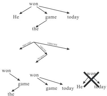
Figure 1: A dependency parse tree (top), one of its feature trees (middle) and some of its subtrees (bottom). He ← won → today is not a subtree becauseHeandtodayare not adjacent siblings.
5 Efficient Candidate Generation 5.1 Polynomial Kernel
As mentioned above, we generate the r + 1 -order candidates by combining the candidates of orderr. An efficient feature generation algorithm should be carefully designed to avoid duplicates, otherwise#f+and#f−may be over counted.
The candidate generation algorithm is kernel dependent. For polynomial kernel, we just combine any twor-order candidates and remove the combined feature if its order is not r + 1. This method requires square running time for each example.
5.2 Dependency Tree Kernel 5.2.1 Definition
Collins and Duffy (2002) proposed tree kernels for constituent parsing which includes the all-subtree features. Similarly, we define dependency tree kernel for dependency parsing. For compatibility with the previously studied subtree features for dependency parsing, we propose a new dependency tree kernel that is different from Culotta and Sorensen’s (Culotta and Sorensen,
2004). Given a dependency parse tree T
concatenation of the POS tags of the head and the modifier, etc.
A feature tree of T is a tree that has the same structure as T, while each arc is replaced by any of its basic features. For a parse tree that has L−1arcs, and each arc hasdbasic features, the number of the feature trees isdL−1. For example,
the dependency parse tree for sentenceHe won the game today is shown in Figure 1. Suppose each arc has two basic features: word pair and POS tag pair. Then there are24 feature trees, because each
arc can be replaced by either word pair or POS tag pair.
A subtree of a tree is a connected fragment in the tree. In this paper, to reduce computational cost, we restrict that adjacent siblings in the subtrees must be adjacent in the original tree. For exampleHe←won→game is a subtree, butHe ←won→todayis not a subtree. The motivation of the restriction is to reduce the number of subtrees, for a node having k children, there are k(k−1)/2subtrees, but without the restriction the
number of subtrees is exponential:2k.
A sub feature tree of a dependency tree T is a feature tree of any of its subtrees. For example, the dependency tree in Figure 1 has 12 subtrees including four arcs, four arc pairs, the three arc triples and the full feature tree, and each subtree having sarcs has 2s sub feature trees. Thus the dependency tree has2∗4+4∗22+3∗23+24 = 64
sub feature trees.
Given two dependency trees T1 and T2, the
dependency tree kernel is defined as the number of common sub feature trees ofT1andT2. Formally,
the kernel function is defined as K(T1, T2) =
∑
n1∈T1,n2∈T2
∆(n1, n2)
where∆(n1, n2)denotes the number of common
sub feature trees rooted inn1andn2nodes.
Like tree kernel, we can calculate ∆(n1, n2)
recursively. Let ci and c′j denote the i-th child of n1 and j-th child of n2 respectively,
let STp,l(n1) denote the set of the sub feature
trees rooted in node n1 and the children of the
root arecp, cp+1, . . . , cp+l−1, we denoteSTq,l(n2)
similarly. Then we define
∆p,q,l(n1, n2) =
∑
p,q
|STp,l(n1)
∩
STq,l(n2)|
the number of common sub feature trees in STp,l(n1)andSTq,l(n2).
a
[image:6.595.361.474.62.158.2]b
Figure 2: For any subtree rooted in a with the rightmost leaf b, we could extend the subtree by any arc below or right to the path from a to b (shown in black)
To calculate∆p,q,l(n1, n2), we first consider the
sub feature trees with only two levels, i.e., sub feature trees that are composed ofn1, n2and some
of their children. We initialize∆p,q,1(n1, n2)with
number of the common features of arcsn1 → cp andn2 → c′q. Then we calculate ∆p,q,l(n1, n2)
recursively using
∆p,q,l(n1, n2)
=∆p,q,l−1(n1, n2)∗∆p+l,q+l,1(n1, n2)
And∆(n1, n2) =∑p,q,l∆p,q,l(n1, n2)
Next we consider all the sub feature trees, we have
∆p,q,l(n1, n2)
=∆p,q,l−1(n1, n2)∗(1 + ∆(cp+l−1, c′q+l−1)
)
Computing the dependency tree kernel for two parse trees requires|T1|2∗ |T2|2∗min{|T1|,|T2|}
running time in the worst case, as we need to enumeratep, q, landn1, n2.
One way to incorporate the dependency tree kernel for parsing is to rerank theKbest candidate parse trees generated by a simple linear model. Suppose there are n training samples, the size of the kernel matrix is (K ∗ n)2, which is
unacceptable for large datasets.
5.2.2 Candidate Generation
feature trees in the kernel space using Algorithm 1. Ther-order features in dependency tree kernel space are the sub feature trees with r arcs. The candidate feature generation in Line 17 has two steps: first we generate the subtrees withr arcs, then we generate the sub feature trees for each subtree.
The simplest way for subtree generation is to enumerate the combinations ofr+ 2words in the sentence, and check if these words form a subtree.
We can speed up the generation by using the results of the subtrees withr+ 1 words (r arcs). For each subtree Sr with r arcs, we can add an extra word toSr and generateSr+1 if the words
form a subtree.
This method has three issues: first, the time complexity is exponential in the length of the sentence, as there are2L combinations of words, Lis the sentence length; second, it may generate duplicated subtrees, and over counts the gradients. For example, there are two ways to generate the subtree He won the game in Figure 1: we can either add wordHeto the subtree won the game, or add wordtheto the subtreeHe won game; third, checking a fragment requiresO(L)time.
These issues can be solved using the well known rightmost-extension method (Zaki, 2002; Asai et al., 2002; Kudo et al., 2005) which enumerates all subtrees from a given tree efficiently. This method starts with a set of trees consisting of single nodes, and then expands each subtree attaching a new node.
Specifically, it first indexes the words in the pre-order of the parse tree. When generating Sr+1,
only the words whose indices are larger than the greatest index of the words inSr are considered. In this way, each subtree is generated only once. Thus, we only need to consider two types of words: (i) the children of the rightmost leaf ofSr, (ii) the adjacent right sibling of the any node inSr, as shown in Figure 2.
The total number of subtrees is no greater than L3, because the level of a subtree is less than L,
and for the children of each node, there are at most L2 subsequences of siblings. Therefore the time
complexity for subtree extraction isO(L3).
6 Experiments
6.1 Experimental Results on English Dataset 6.1.1 Settings
First we used the English Penn Tree Bank (PTB) with standard train/develop/test for evaluation. Sections 2-21 (around 40K sentences) were used as training data, section 22 was used as the development set and section 23 was used as the final test set.
We extracted dependencies using Joakim Nivre’s Penn2Malt tool with Yamada and Matsumoto’s rules (Yamada and Matsumoto, 2003). Unlabeled attachment score (UAS) ignoring punctuation is used to evaluate parsing quality.
We apply our technique to rerank the parse trees generated by a third order parser (Koo and Collins, 2010) trained using 10 best MIRA algorithm with 10 iterations. We generate the top 10 best candidate parse trees using10fold cross validation for each sentence in the training data. The gold parse tree is added if it is not in the candidate list. Then we learn a reranking model using these candidate trees. During testing, the score for a parse tree T is a linear combination of the two models:
score(T) =βscoreO3(T) +scorererank(T)
where the meta-parameter β = 5 is tuned by grid search using the development dataset. scoreO3(T)andscorererank(T)are the outputs of the third order parser and the reranking classifier respectively.
For comparison, we implement the following reranking models:
• Perceptron with Polynomial kernels
K(a,b) = (aTb+ 1)d,d= 2,4,8 • Perceptron with Dependency tree kernel. • Perceptron with features generated by
templates, including all siblings and fourth order features.
• Perceptron with the features selected in polynomial and tree kernel spaces, where thresholdC= 3.
whwm, phpm, whpm, phwm
ph−1pm, ph−1wm,phpm−1, whpm−1 ph+1pm, ph+1wm,phpm+1, whpm+1 ph−1phpm, phph+1pm, phpm−1pm, phpmpm+1
Concatenate features above with length and direction phpbpm
Table 1: Basic features in polynomial and dependency tree kernel spaces, wh: the word of head node,wmdenotes the word of modifier node, ph: the POS of head node, pm denotes the POS of modifier node,ph+1: POS to the right of head
node, ph−1: POS to the left of modifier node,
pm+1: POS to the right of head node,pm−1: POS
to the left of modifier node,pb: POS of a word in between head and modifier nodes.
[image:8.595.307.527.62.304.2]direction of the arcs, and the POS tags of the words lying between the head and modifier, as shown in Table 1. The POS tags are automatically generated by 10 fold cross validation during training, and a POS tagger trained using the full training data during testing which has an accuracy of96.9%on the development data and97.3%on the test data.
As kernel methods are not scalable for large datasets, we applied the strategy proposed by Collins and Duffy (2002), to break the training set into 10chunks of roughly equal size, and trained
10separate kernel perceptrons on these data sets. The outputs from the 10 runs on test examples were combined through the voting procedure.
For feature selection, we set the maximum iteration numberM = 100. We use the first order and second order features for pre-training. We choose the constant step sizeαt = 1because we find this could quickly reduce the prediction error in very few iterations.
We use the SHA-1 hash function to generate the hash codes for the spectral bloom filter. The SHA-1 hash function produces a 160-bit hash code for each candidate feature. The hash code is then segmented into 5 segments, in this way we get five hash codesh1, . . . , h5. Each code has 32 bits.
Then we create232(4G) counters. The threshold
θ is set to3, thus each counter requires 2bits to store the counts. The spectral bloom filter costs
1Gmemory in total.
Furthermore, to reduce memory cost, we save the local data structure such as the selected features in Step 15 of Algorithm 1 whenever possible, and load them into the memory when needed.
After feature selection, we did not use the L1
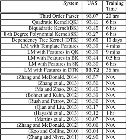
System UAS Training Time Third Order Parser 93.07 20 hrs Quadratic Kernel(QK) 93.41 6 hrs Biquadratic Kernel(BK) 93.45 6 hrs 8-th Degree Polynomial Kernel(8K) 93.27 6 hrs
Dependency Tree Kernel (DTK) 93.65 10 days LM with Template Features 93.39 4 mins
LM with Features in QK 93.39 9 mins LM with Features in BK 93.44 0.5 hrs LM with Features in 8K 93.30 6 hrs LM with Features in DTK 93.72 36 hrs (Zhang and McDonald, 2014) 93.57 N/A
(Zhang et al., 2013) 93.50 N/A (Ma and Zhao, 2012) 93.40 N/A (Bohnet and Kuhn, 2012) 93.39 N/A (Rush and Petrov, 2012) 93.30 N/A (Qian and Liu, 2013) 93.17 N/A (Hayashi et al., 2013) 93.12 1 hr (Martins et al., 2013) 93.07 N/A (Zhang and McDonald, 2012) 93.06 N/A (Koo and Collins, 2010) 93.04 N/A (Zhang and Nivre, 2011) 92.90 N/A
Table 2: Comparison between our system and the state-of-art systems on English dataset. LM is short for Linear Model, hrs, mins are short for hours and minutes respectively
SVM for testing, instead, we trained an averaged perceptron with the selected features. Because we find that the averaged perceptron significantly outperformsL1SVM.
6.1.2 Results
Experimental results are listed in Table 2, all systems run on a 64 bit Fedora operation system with a single Intel core i7 3.40GHz and 32G memory. We also include results of representative state-of-the art systems.
It is clear that the use of kernels or the deep features in kernel spaces significantly improves the baseline third order parser and outperforms the reranking model with shallow, template-generated features. Besides, our feature selection outperforms kernel methods in both efficiency and accuracy.
It is unsurprising that the dependency tree kernel outperforms polynomial kernels, because it captures the structured information. For example, polynomial kernels can not distinguish the grand-child feature or sibling feature from the combination of two separated arc features.
When no additional resource is available, our parser achieved the best reported performance
C #Feat #Template Hours Mem(G) UAS 1 0.34G N/A stalled OOM N/A 2 0.34G N/A stalled OOM N/A 3 33.1M 11.4K 36 4.0 93.72
5 6.32M 2.1K 20 2.2 93.55
[image:9.595.346.488.61.136.2]10 2.10M 1.6K 5 1.4 93.40
Table 3: Feature selection in dependency kernel space with different thresholdC.
worth pointing that our method is orthogonal to other reported systems that benefit from advanced inference algorthms, such as cube pruning (Zhang and McDonald, 2014), AD3(Martins et al., 2013),
etc. We believe that combining our techniques with others’ will achieve further improvement.
Reranking the candidate parse trees of 2416 testing sentences takes 67 seconds, about 36 sentences per second.
To further understand the complexity of our algorithm, we perform feature selection in dependency tree kernel space with different thresholds C and record the number of selected features and feature templates, the speed and memory cost. Table 3 shows the results. We can see that our algorithm works efficiently when C ≥ 3, but for C < 3, the number of selected features grows drastically, and the program runs out of memory (OOM).
6.2 Experimental Results on CoNLL 2009 Dataset
Now we looked at the impact of our system on non-English treebanks. We evaluate our system on six other languages from the CoNLL 2009 shared-task. We used the best setting in the previous experiment: reranking model is trained using the features selected in the dependency tree kernel space. For POS tag features we used the predicted tags.
As the third order parser can not handle non-projective parse trees, we used the graph transformation techniques to produce non-projective structures (Nivre and Nilsson, 2005). First, the training data for the parser is projectivized by applying a number of lifting operations (Kahane et al., 1998) and encoding information about these lifts in arc labels. We used the path encoding scheme where the label of each arc is concatenated with two binary tags, one indicates if the arc is lifted, the other indicates if the arc is along the lifting path from the syntactic to the linear head. Then we train a projective
Language Ours Official Best Chinese 76.77 79.17
Japanese 92.68 92.57
German 87.40 87.48
Spanish 87.82 87.64
Czech 80.51 80.38
Catalan 86.98 87.86
Table 4: Experimental Results on CoNLL 2009 non-English datasets.
parser on the transformed data without arc label information and a classifier to predict the arc labels based on the projectivized gold parse tree structure. During testing, we run the parser and the classifier in a pipeline to generate a labeled parse tree. Labeled syntactic accuracy is reported for comparison.
Comparison results are listed in Table 4. We achieved the best reported results on three languages, Japanese, Spanish and Czech. Note that CoNLL 2009 also provide the semantic labeling annotation which we did not used in our system. While some official systems benefit from jointly learning parsing and semantic role labeling models.
7 Conclusion
In this paper we proposed a new feature selection algorithm that selects features in kernel spaces in a coarse to fine order. Like frequent mining, the efficiency of our approach comes from the anti-monotone property of the subgradients. Experimental results on the English dependency parsing task show that our approach outperforms standard kernel methods. In the future, we would like to extend our technique to other real valued kernels such as the string kernels and tagging kernels.
Acknowledgments
[image:9.595.72.297.61.127.2]References
Tatsuya Asai, Kenji Abe, Shinji Kawasoe, Hiroki Arimura, Hiroshi Sakamoto, and Setsuo Arikawa. 2002. Efficient substructure discovery from large semi-structured data. InProceedings of the Second SIAM International Conference on Data Mining,
Arlington, VA, USA, April 11-13, 2002, pages 158–
174.
Burton H. Bloom. 1970. Space/time trade-offs in hash coding with allowable errors. Commun. ACM, 13(7):422–426, July.
Bernd Bohnet and Jonas Kuhn. 2012. The best of bothworlds – a graph-based completion model for transition-based parsers. InProc. of EACL.
S. Boyd and A. Mutapcic. 2006. Subgradient methods.
notes for EE364.
Saar Cohen and Yossi Matias. 2003. Spectral bloom filters. InProc. of SIGMOD, SIGMOD ’03.
Michael Collins and Nigel Duffy. 2002. New ranking algorithms for parsing and tagging: Kernels over discrete structures, and the voted perceptron. In
Proc. of ACL, ACL ’02.
Aron Culotta and Jeffrey Sorensen. 2004. Dependency tree kernels for relation extraction. InProc. of ACL, ACL ’04.
Katsuhiko Hayashi, Shuhei Kondo, and Yuji Matsumoto. 2013. Efficient stacked dependency parsing by forest reranking. TACL, 1.
Sylvain Kahane, Alexis Nasr, and Owen Rambow. 1998. Pseudo-projectivity, a polynomially parsable non-projective dependency grammar.
In Proceedings of the 36th Annual Meeting of the
Association for Computational Linguistics and 17th International Conference on Computational
Linguistics, Volume 1, pages 646–652, Montreal,
Quebec, Canada, August. Association for Computational Linguistics.
Terry Koo and Michael Collins. 2010. Efficient third-order dependency parsers. InProc. of ACL.
Taku Kudo, Jun Suzuki, and Hideki Isozaki. 2005. Boosting-based parse reranking with subtree features. In Proceedings of the 43rd Annual Meeting of the Association for Computational
Linguistics (ACL’05), pages 189–196, Ann Arbor,
Michigan, June. Association for Computational Linguistics.
Zhiyun Lu, Avner May, Kuan Liu, Alireza Bagheri Garakani, Dong Guo, Aur´elien Bellet, Linxi Fan, Michael Collins, Brian Kingsbury, Michael Picheny, and Fei Sha. 2014. How to scale up kernel methods to be as good as deep neural nets. CoRR, abs/1411.4000.
Xuezhe Ma and Hai Zhao. 2012. Fourth-order dependency parsing. In Proceedings of
COLING 2012: Posters, pages 785–796, Mumbai,
India, December. The COLING 2012 Organizing Committee.
Andre Martins, Miguel Almeida, and Noah A. Smith. 2013. Turning on the turbo: Fast third-order non-projective turbo parsers. InProc. of ACL.
Joakim Nivre and Jens Nilsson. 2005. Pseudo-projective dependency parsing. In Proceedings of the 43rd Annual Meeting on Association for
Computational Linguistics, ACL ’05, pages 99–
106, Stroudsburg, PA, USA. Association for Computational Linguistics.
Daisuke Okanohara and Jun’ichi Tsujii. 2009. Learning combination features with l1 regularization. InProceedings of Human Language Technologies: The 2009 Annual Conference of the North American Chapter of the Association for Computational Linguistics, Companion Volume:
Short Papers, pages 97–100, Boulder, Colorado,
June. Association for Computational Linguistics.
Xian Qian and Yang Liu. 2013. Branch and bound algorithm for dependency parsing with non-local features. TACL, 1.
Alexander Rush and Slav Petrov. 2012. Vine pruning for efficient multi-pass dependency parsing. In
Proc. of NAACL. Association for Computational
Linguistics.
Jun Suzuki, Hideki Isozaki, and Eisaku Maeda. 2004. Convolution kernels with feature selection for natural language processing tasks. InProceedings of the 42nd Meeting of the Association for
Computational Linguistics (ACL’04), Main Volume,
pages 119–126, Barcelona, Spain, July.
Mingkui Tan, Ivor W. Tsang, and Li Wang. 2012. Towards large-scale and ultrahigh dimensional feature selection via feature generation. CoRR, abs/1209.5260.
Ben Taskar. 2004. Learning Structured Prediction
Models: A Large Margin Approach. Ph.D. thesis,
Stanford University.
Christopher K. I. Williams and Matthias Seeger. 2001. Using the nystr¨om method to speed up kernel machines. InNIPS.
Yu-Chieh Wu, Jie-Chi Yang, and Yue-Shi Lee. 2007. An approximate approach for training polynomial kernel svms in linear time. InProc. of ACL, ACL ’07.
Mohammed J. Zaki. 2002. Efficiently mining frequent trees in a forest. InProceedings of the Eighth ACM SIGKDD International Conference on Knowledge
Discovery and Data Mining, KDD ’02, pages 71–
80, New York, NY, USA. ACM.
Hao Zhang and Ryan McDonald. 2012. Generalized higher-order dependency parsing with cube pruning.
InProc. of EMNLP.
Hao Zhang and Ryan McDonald. 2014. Enforcing structural diversity in cube-pruned dependency parsing. InProc. of ACL.
Yue Zhang and Joakim Nivre. 2011. Transition-based dependency parsing with rich non-local features. In
Proc. of ACL-HLT.
Qi Zhang, Fuliang Weng, and Zhe Feng. 2006. A progressive feature selection algorithm for ultra large feature spaces. InProc. of ACL.