M. M. Scase1,∗ K. A. Baldwin2, and R. J. A. Hill3
1
School of Mathematical Sciences, University of Nottingham, Nottingham NG7 2RD, UK
2
Faculty of Engineering, University of Nottingham, Nottingham NG7 2RD, UK
3
School of Physics and Astronomy, University of Nottingham, Nottingham NG7 2RD, UK
(Dated: November 7, 2016)
The effect of rotation upon the classical Rayleigh-Taylor instability is considered. We consider a two-layer system with an axis of rotation that is perpendicular to the interface between the layers. In general we find that a wave mode’s growth rate may be reduced by rotation. We further show that in some cases, unstable axisymmet-ric wave modes may be stabilized by rotating the system above a critical rotation rate associated with the mode’s wavelength, the Atwood number and the flow’s aspect ratio.
I. INTRODUCTION
Understanding of the Rayleigh-Taylor instability has increased progressively since Lord Rayleigh’s [16] initial work and the investigations of Taylor [24] and Lewis [9]. The motivation for research into this fundamental prob-lem has changed over time, from the original interests of Taylor and Lewis to the energy supply and astrophysical aspects of more recent work. The now familiar struc-ture of the Rayleigh-Taylor instability has been observed from small scales in, for example, inertial confinement fusion problems [see e.g., 5], to extremely large scales, such as the crab nebula [see, e.g., 25] where pulsar winds accelerate through dense supernova remnants. In many cases of practical interest, it would be desirable to have some further control over the instability after the setting of the initial density profiles. One possibility is to ro-tate the system; the often stabilising effect of rotation on a flow is well-known [see e.g., 6]. Tao et al. [21] investigated whether rotation may be used to influence the Rayleigh-Taylor instability at the surface of an iner-tial confinement fusion target by considering instability at an interface parallel to the axis of rotation. In iner-tial confinement fusion, the Rayleigh-Taylor instability reduces the efficiency of fusion during both the accelera-tion phase, between the ablator and the fuel, and during the deceleration phase, between the hot and cold fuel re-gions [see e.g., 11]. The efficiency is reduced due to the increased interfacial surface area between the two layers in each case. The work of Tao et al. [21] suggested that the instability may be suppressed around the equatorial region of a spherical rotating target.
In a previous paper [1] we reported results of experi-ments to study the development of the Rayleigh-Taylor
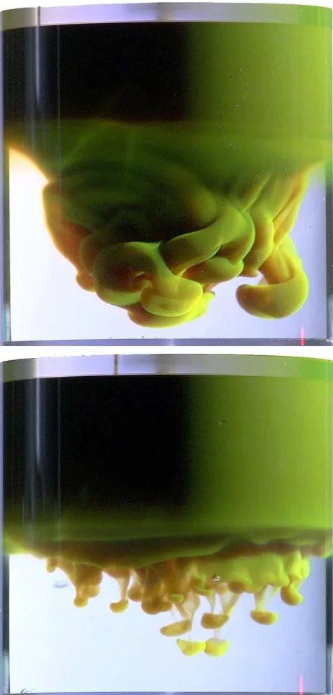
instability in a two-layer fluid system with axis of tion perpendicular to the layers. The presence of rota-tion introduces a restoring force on fluid elements moving perpendicular to the axis of rotation: the Coriolis force. This fictitious force, which appears in a rotating refer-ence frame, acts to restore a fluid element, traveling in a direction perpendicular to the axis of rotation, to its orig-inal position, following a curved path. The presence of the Coriolis force therefore allows the fluid to support ertial wave motions, the rotational counterpart to the in-ternal gravity waves supported by a density stratification [see e.g., 17, 18]. As will be shown, the Coriolis force acts to inhibit large-scale overturning motions at the unstable interface and is consequently important in changing the character of the developing Rayleigh-Taylor instability as the rate of rotation is increased. The effect is shown qualitatively in Fig. 1. It can be seen that the large-scale overturning motion required to form large vortices (top) is restricted in the presence of rotation (bottom).
In this paper we present a theoretical study of the Rayleigh-Taylor instability under the influence of rota-tion. Miles [12, 13] considered the effects of rotation on infinitesimal free-surface waves on a body of water, remarking on Fultz’s [6] observation that the parabolic nature of the free-surface is important and cannot be ne-glected as previous authors had [see, e.g., 8]
‘The planar [horizontal hydrostatic interface] approximation is necessarily inconsistent for axisymmetric gravity waves in the sense that both the rotation induced shift . . . and the free-surface slope are of the same order of magnitude.’
FIG. 1: The upper image, taken of our experiments, is of a magnetically induced Rayleigh-Taylor instability
developing in a non-rotating system. The instability develops in time, forming large vortices that transport
the green fluid downwards. The lower image is of the same fluids but here the system is rotating. The effect
of the rotation can be seen to restrict the size of the vortices that form and inhibit the bulk vertical transport of fluid. The times shown are 1.92 s and 3.52 s
after initiation in the upper and lower images respectively. The experiments are described in [1, 19].
The tank diameter is 90 mm, and the rotation rate in the lower image was 2.52 rad s−1.
there is a strong dependence on the aspect ratio of the layers.
In§II we develop an inviscid theory based on the previ-ous theories of Rayleigh-Taylor instability due to Taylor [24] and the modeling of surface oscillations on rotating bodies of fluid due to Lamb [8] and Miles [12, 13]. The key results are: a dispersion relation for axisymmetric and asymmetric perturbations to the interface of a ro-tating two-layer fluid system (both stable and Rayleigh-Taylor unstable); a critical rotation rate for stabilizing Rayleigh-Taylor unstable axisymmetric modes of pertur-bation. In§III we discuss our results and draw our con-clusions.
II. MODELING II.1. Growth of the instability
We begin by considering a two-layer rotating fluid as shown in Fig. 2. The upper layer is denoted by a sub-script 1 and the lower layer by a subsub-script 2. We assume cylindrical polar coordinates with unit vectors er, eθ,
and ez in the radial, azimuthal, and vertical directions respectively and take the rotation to be described by the pseudovector Ω = Ωez. The radius of the cylinder is
a, and the lid and base of the cylinder are at z = ±d. The whole system may be accelerated vertically at a rate
g1. Ignoring the effects of viscosity, we write the rotating Euler equation for the fluid in each layer as
Duj Dt =−
1
ρj
∇pj+g∗−Ω×(Ω×x)−2Ω×uj, (1)
forj = 1,2, whereg∗ =−(g+g1)ez and uj and xare velocity and position vectors respectively, in the rotating frame. For simplicity we drop the g1 notation and will write g∗ = −gez, with the understanding that g may not be equal to the acceleration due to gravity, and may change sign as a result of external bulk acceleration of the system. When the fluid system is spun up into a hydrostatic regime (in the rotating, non-inertial reference frame) thenuj≡0and
pj =p0−ρj
gz−Ω 2
2 (r 2−1
2a 2)
, j= 1,2, (2)
where p0 is a constant reference pressure equal to the pressure at the interface when the system is not rotating. We take z = z0(r) to be the position of the interface between the two fluid layers. In the absence of viscosity, requiring the stress to be continuous across the interface is equivalent to requiring continuity of pressure across the interface. Hence we may writep1=p2onz=z0(r), and it follows that the interface is an isobar on whichpj=p0 and has profile given by
z0(r) =
Ω2(r2−1 2a2)
g
z=z0(r)
Ω
g1
u2,ρ2
u1,ρ1
0 a
D1
D2
−d
[image:3.612.64.288.61.310.2]0 d
FIG. 2: Two layers of incompressible fluid of densityρ1 andρ2occupy a cylindrical tank of radiusathat is being accelerated [see 24] at a rateg1. When the tank is
not rotating we take the interface between the fluids to be atz= 0 (coordinates moving with the tank), the base of the tank atz=−dand the lid of the tank at
z=d. The tank is spun up to have a constant angular velocity Ω about the z-axis. The isobar describing the
interface is given byz=z0(r) where
z0(r) = Ω2(r2−12a2)/(2g) andp=p0 onz=z0(r). The meridional plane is split into two domains,D1 andD2
representing the upper and lower layers respectively (shaded gray).
constrained by Ra
0 z0(r)rdr= 0 to ensure that the fluid layers are of equal depth. The shape and position of the interface are independent of the densities of the fluid in the upper and lower layers. Hence, whilst the value ofp0 and the stability of the interface may change according as to whetherρ1< ρ2orvice-versa, the profile remains the familiar ‘concave’ paraboloid such as may be observed at the free surface of a vigorously stirred beverage.
Following Taylor [24] we investigate the development of the Rayleigh-Taylor instability under rotation by con-sidering the development of a perturbation to the in-terface. The strength of a stratification can be char-acterized by an Atwood number, defined here as A =
(ρ2−ρ1)/(ρ2+ρ1). Using this definition we have that for a stable stratificationA >0 and for an unstable
stratifi-cationA <0 [n.b., in experimental investigations of the
Rayleigh-Taylor instability, many authors, dealing only with unstable flows, define the Atwood number with op-posite sign]. The amplitude of the perturbation and the velocity and pressure deviation from the hydrostatic are all assumed to be small. We describe the fluid velocity
and pressure perturbations in terms of a scalar poten-tial, unifying the approaches of Taylor [24], in modeling the non-rotating Rayleigh-Taylor instability, and Miles [12, 13], in modeling surface waves on a rotating fluid. Taylor [24] used a standard velocity potential and Miles [13] used an ‘acceleration potential’ of the kind proposed by Poincar´e [14]. Here we make use of the ‘generalized potential’ described by Hart [7]. Specifically, for an in-terface perturbation
z=z0(r) +ǫ ζ(r, θ, t), (4)
whereǫ|ζ| ≪d, we take the velocity perturbation to the hydrostatic background to be
uj=ǫ
(
1 + 1 4Ω2
∂2
∂t2
∇φj− 1 2Ω
∂
∂t(ez×∇φj)
+ez×(ez×∇φj)
)
, (5)
forj = 1,2, and the pressure to be
pj =p0−ρjg[z−z0(r)]−ǫρj
∂φj
∂t +
1 4Ω2
∂3φ j
∂t3
, (6)
forj = 1,2.
Substitution of (5) and (6) into (1) shows that the ro-tating Euler equation is satisfied at leading order by the order 1 hydrostatic pressure terms and at orderǫby the generalized potentialφ. (We note that both the present formulation, and that of Miles [12, 13], necessarily im-ply a swirl component to the flow as soon as the radial velocity is non-zero.) By further assuming that the fluid in each layer is incompressible, i.e.,∇ ·uj= 0, we obtain the governing wave equation for each fluid layer
∂t2∇2+ 4Ω2∂z2 φj= 0, j= 1,2. (7)
Solutions to this type of wave equation in the context of inertial waves and internal gravity waves are well-known [see, e.g., 10, and references therein].
We seek to solve the governing equation (7) together with the following boundary conditions: that there is no flow through the tank walls, an impermeability condition given by
u·er= 0, onr=a, u·ez= 0, onz=±d.
(8)
We also require that the velocity on the axis of rotation,
r= 0, is sufficiently regular, specifically that
r∂φ2j/∂r→0 asr→0, (9)
(this condition allows for finite fluid velocities across the axis of rotation); and finally, we require continuity of stress across the interface. In the absence of viscosity we therefore require
p
+
Since ζ is unknown we require the kinematic condition that the interface moves with the local fluid velocity to close the system:
D
Dt(z0+ǫζ) =u·ez, onz=z0(r) +ǫζ(r, θ, t). (11)
Following Taylor [24] and Miles [13] we adopt a vari-ational formulation and seek normal mode solutions of the form
φ= ˆφ(r, z) exp{i (ωt+mθ)}, ζ= ˆζ(r) exp{i (ωt+mθ)},
(12) wherem∈N0is an azimuthal wavenumber. Substitution into (7) yields the governing equation
1
r ∂ ∂r r
∂φˆj
∂r
!
−m 2
r2 φˆj+ 1−µ 2∂
2φˆ j
∂z2 = 0, j= 1,2, (13) where we adopt Miles’ [13] notation by defining µ = 2Ω/ω. The boundary conditions (8) and (9) become
r∂φˆ2
j/∂r→0 as r→0,
r∂φˆj/∂r+µmφˆj= 0, onr=a,
∂φˆj/∂z= 0, onz=±d,
(14)
where the plus or minus is taken according to whetherj= 1 or 2 respectively. The condition of pressure continuity across the interface (10) yields at orderǫ
iωµ2ζˆ=2Ω 2
g
1− 1
µ2
1 +A
A φˆ2−
1−A
A φˆ1
,
(15) on z = z0(r). The kinematic condition (11) at order ǫ can be written as
iωµ2ζˆ=z′ 0
∂φˆj
∂r + µm
r φˆj
!
− 1−µ2∂φˆj
∂z, j= 1,2,
(16) onz=z0(r) for each layer, wherez′0≡dz0/dr.
The variational functional Φ[ ˆφ1,φˆ2] is defined by mul-tiplying the governing equation (13) by ρjφˆj and inte-grating over the domain D =D1∪D2 = [0, a]×[−d, d]
(see Fig. 2) so that
Φ =
Z
D
ρφˆ
(
1
r ∂ ∂r r
∂φˆ ∂r
!
−m 2
r2 φˆ+ (1−µ 2)∂2φˆ
∂z2
)
dA.
(17) Following the method outlined in Miles [13] we write the integral (17) in conservative form giving
Φ = Z D ρ " 1 r ∂ ∂r rφˆ
∂φˆ ∂r
!
+ (1−µ2) ∂
∂z φˆ ∂φˆ ∂z !# dA − Z D ρ
∂φˆ ∂r
!2
+m 2
r2 φˆ
2+ (1−µ2) ∂φˆ
∂z
!2
dA.
(18)
We consider the first integral in (18) and integrate over
D1andD2separately. DefiningI1to be the integral over D1 andI2 to be the integral overD2, we have
I1=
Z z0(a)
z0(0)
Z r0(z)
0
ρ1
r ∂ ∂r rφˆ1
∂φˆ1
∂r
!
rdrdz
+
Z d
z0(a)
Z a
0
ρ1
r ∂ ∂r rφˆ1
∂φˆ1
∂r
!
rdrdz
+
Z a
0
Z d
z0(r)
ρ1(1−µ2)
∂ ∂z φˆ1
∂φˆ1
∂z
!
rdzdr, (19)
wherer0(z) is the well-defined inverse ofz0(r). Integrat-ing and enforcIntegrat-ing the boundary conditions∂φˆ1/∂z|z=d= 0, (r∂φˆ1/∂r+µmφˆ1)|r=a= 0, andr∂φˆ21/∂r→0 asr→0 implies
I1=ρ1
Z z0(a)
z0(0)
rφˆ1
∂φˆ1
∂r r=r 0(z) dz
−ρ1µm
Z d
z0(a) ˆ
φ21
r=adz
−ρ1(1−µ2)
Z a
0 ˆ
φ1
∂φˆ1
∂z
z=z0(r)
rdr. (20)
Transforming the first term in (20) by making the sub-stitutionz=z0(r) gives the result
I1=−ρ1µm
Z d
z0(a) ˆ
φ2 1
r=adz
+ρ1
Z a 0 ˆ φ1 ( z′ 0
∂φˆ1
∂r −(1−µ
2)∂φˆ1
∂z ) z=z 0(r)
rdr.
(21a)
Following a similar procedure, we may also show
I2=−ρ2µm
Z z0(a)
−d ˆ φ2 2 r=adz
−ρ2
Z a 0 ˆ φ2 ( z′ 0
∂φˆ2
∂r −(1−µ
2)∂φˆ2
∂z ) z=z 0(r)
rdr.
(21b)
Eliminating the interface perturbation,ζ, from the pres-sure continuity condition (15) and the kinematic condi-tion (16) we see that
z′ 0
∂φˆj
∂r −(1−µ
2)∂φˆj
∂z =−z
′ 0
µm r φˆj
+2Ω 2
g
1− 1
µ2
1 +A
A φˆ2−
1−A
A φˆ1
, (22)
as
I1=−ρ1µm
Z d
z0(a) ˆ
φ2 1
r=adz
+
Z a
0
ρ1φˆ1
2Ω2
g
1− 1
µ2
1 +A
A φˆ2−
1−A
A φˆ1
−z′ 0
µm r φˆ1
o
z=z0(r)
rdr, (23a)
I2=−ρ2µm
Z z0(a)
−d ˆ φ2 2 r=adz
−
Z a
0
ρ2φˆ2
2Ω2
g
1− 1
µ2
1 +A
A φˆ2−
1−A
A φˆ1
−z′ 0
µm r φˆ2
o
z=z0(r)
rdr. (23b)
Substituting (23) into (18) we have that
Φ[φ1, φ2] =−ρ1µm
Z d
z0(a) ˆ
φ21
r=adz
+
Z a
0
ρ1φˆ1
2Ω2
g
1− 1
µ2
1 +A
A φˆ2−
1−A
A φˆ1
−z′ 0
µm r φˆ1
o z=z
0(r)
rdr−ρ2µm
Z z0(a)
−d ˆ
φ22
r=adz
−
Z a
0
ρ2φˆ2
2Ω2
g
1− 1
µ2
1 +A
A φˆ2−
1−A
A φˆ1
−z′ 0
µm r φˆ2
o
z=z0(r)
rdr
− Z D1 ρ1
∂φˆ1
∂r
!2
+m 2
r2 φˆ 2
1+ (1−µ2)
∂φˆ1
∂z
!2 dA
− Z D2 ρ2
∂φˆ2
∂r
!2
+m 2
r2 φˆ 2
2+ (1−µ2)
∂φˆ2
∂z
!2 dA.
(24)
Taking the functional derivative of Φ with respect to, for example, ˆφ1, where δ1Φ ≡ Φ[ ˆφ1+δφˆ1,φˆ2]−Φ[ ˆφ1,φˆ2] yields, after some manipulation,
δ1Φ = 2ρ1
Z D1 ( 1 r ∂ ∂r r
∂φˆ1
∂r
!
−m 2
r2 φˆ1+ 1−µ 2∂
2φˆ 1
∂z2
)
δφˆ1dA
−2ρ1
Z d
z0(a)
(
µmφˆ1+r
∂φˆ1
∂r
)
δφˆ1
r=a dz
+ 2ρ1
Z a 0 2Ω2 g
1− 1
µ2
1 +A
A φˆ2−
1−A
A φˆ1
−z′ 0
µm r φˆ1−
"
z′ 0
∂φˆ1
∂r −(1−µ
2)∂φˆ1
∂z
#)
δφˆ1
z=z 0(r)
rdr.
(25)
So we see that the functional Φ is stationary with respect to first-order variations of ˆφ1 about the solution of the governing equation (13) in D1, the boundary condition
(22) forj = 1 at the interface z =z0(r) and at the no-radial flow condition atr = a on the boundary of D1.
Similarly, Φ is stationary with respect to first-order vari-ations of ˆφ2about the solution of the governing equation (13) in D2, the boundary condition (22) for j = 2 at
the interfacez =z0(r) and the no-radial flow condition at r =a on the boundary of D2. (The Euler-Lagrange
equation for Φ as expressed in (17) is the governing equa-tion (13) multiplied by 2ρj.) Following Miles [13] we pose trial solutions that satisfy the governing equation (13), the regularity condition atr= 0 and the boundary conditions onr=aand z=±dexactly, and invoke the variational principle only in respect to the final boundary condition onz=z0(r).
If ˆφis an exact solution of the governing equation (13), it follows from the definition of Φ that Φ( ˆφ) = 0. There-fore, if ˆφ is a solution of (13), it follows from (18) and (21) that Z D ρ
∂φˆ ∂r
!2
+m 2
r2 φˆ
2+ (1−µ2) ∂φˆ
∂z
!2
dA=
−ρ1µm
Z d
z0(a) ˆ
φ21
r=adz−ρ2µm Z z0(a)
−d ˆ
φ22
r=adz
+
Z a
0
ρ1φˆ1
(
z′ 0
∂φˆ1
∂r −(1−µ
2)∂φˆ1
∂z )
z=z0(r)
rdr
−
Z a
0
ρ2φˆ2
(
z′ 0
∂φˆ2
∂r −(1−µ
2)∂φˆ2
∂z ) z=z 0(r)
rdr. (26)
Substituting (26) into (24) we therefore have, after sim-plification Φ∝ Z a 0 ( ω2
1 +A
A φˆ2−
1−A
A φˆ1
2
+
Ω2 1−µ2
r ∂
∂r+ 2µm
−g ∂ ∂z
1 +A
A φˆ
2 2−
1−A
A φˆ
2 1 z=z 0(r)
rdr. (27)
The constant of proportionality is (ρ2−ρ1)(1−µ2)/4g, but as interest is focussed upon stationary values of Φ, it will be disregarded. The expression in (27) is the two-layer equivalent of the functional given in (3.2) of Miles [13] and it can be seen that Miles’ expression is recovered in the limit A = 1 (the stable single layer limit). The
cross term in the first term of the integrand is crucial in coupling the behavior of the two fluid layers.
Again, following Miles [13], we seek to construct a series solution based on trial solutions of the form
ˆ
φjn(r, z) =Jm
k
nr
a
cosh kn
a
[z∓d]
p
1−µ2
!
forn= 1,2, . . ., whereJmis a Bessel function of the first kind and we take the minus or plus sign in (28) according to whether j = 1 or 2 respectively. The trial solutions (28) satisfy both the governing equation (13) and the vertical impermeability boundary conditions atz =±d. The radial impermeability boundary condition at r=a
sets the possible modes of solution and so in general we sum over the countable number of solutions,kn, of
kJm+1(k) =m(1 +µ)Jm(k), (29)
which follows from substituting (28) into (14) and setting
r = a. (The ratio kn/a may be regarded as the radial wavenumber associated with the nth mode.) The trial solutions (28) form a complete set over D (and are
or-thogonal in each layer whenµ= 0), and so as the number of terms in the series increases we approach a full solution [13]. (See Finlayson [4] for a description of this classi-cal approach, and its relation to the method of weighted residuals.) Thus, we approximate ˆφ1and ˆφ2 by
ˆ
φj≈φˆ(Nj )= N
X
n=1
cjnφˆjn, j= 1,2, for some N >1.
(30) We adopt a variational approach applied to (27) in order to find the coefficients cjn such that our solution sat-isfies (22) on z = z0(r), the remaining unsatisfied con-dition. Specifically, by seeking stationary values of the functional Φ, by taking the partial derivatives∂Φ/∂cjn,
j= 1,2,n= 1, . . . , N, we may construct 2N linear equa-tions in the 2N coefficients. The eigenvalue equation for
ω is found by setting the determinant of this linear sys-tem to be zero. Ifω has a negative imaginary part then (12) implies growth, and the onset of the Rayleigh-Taylor instability.
In the remainder of§II we initially consider purely ax-isymmetric instabilities, first asymptotically for low ro-tation rates in§II.2.1–II.2.3, and then numerically for ar-bitrary rotation rates in§II.2.4. We then consider asym-metric instabilities, firstly asymptotically for low rotation rates in§II.3.1–II.3.3, and then numerically for arbitrary rotation rates in§II.3.4 and§II.3.5.
II.2. Axisymmetric instability,m= 0
In the first instance we consider purely axisymmetric motion: the special casem = 0. Settingm = 0 in (29) shows that we sum over the zeros ofJ1(k), which implies
k∈R.
II.2.1. Single mode, low rotation rate, gravity wave solutions: asymptotics
Following Miles [13], we initially consider a solution containing a single trial solution each in the upper and lower layers. We further assume a low rotation rate such thatα= Ω2a/g≪1. Using such an approximation Miles
was able to explain the discrepancies between the theory of Lamb [8] and the experimental observations of Fultz [6, Fig. 12] and so we adopt this level of approximation for initial investigation. Seeking an asymptotic expres-sion for the eigenvalue equation forω, we take (28) for some single n ∈ N. By considering ∂Φ/∂c1n = 0 and
∂Φ/∂c2n= 0, and expanding in powers of αwe find, af-ter some significant manipulation, that an eigenvector of the solution is
c∝ 1,−1−16coth(knδ)α+O(α2), (31)
whereδ=d/a, and the eigenvalue equation forω is
ω2∼gAkn
a tanh(knδ) + 2Ω
2[1 + 2k
nδcsch(2knδ)
−1 24k
2
nA2sech 2
(knδ)
+g
aO(α
2). (32)
We observe therefore that if gA < 0 then ω2 <0 and interfacial perturbations will grow rather than oscillate – the Rayleigh-Taylor instability. The form of (32) sug-gests we may be able to suppress this growth to some extent by rotating the system, i.e., the second term in (32) may be used to compete with the first if it has the opposing sign. However, it would be mistaken to suggest that (32) implies that given a sufficient rotation rate an unstable mode could be fully stabilized (ω2 > 0), as is concluded erroneously by Sharma et al. [20] in the con-text of particle laden Rayleigh-Taylor instability. The ex-pansion (32) is asymptotic and its validity breaks down when the second term is comparable to the first. The cor-rect approach is to consider an expansion whenω, not Ω, is small compared to (a/g)1/2(see §II.2.3). The expres-sion in (32) is the first of two key results we present. It is the dispersion relation for a slowly rotating two-layer fluid system that may be either stably stratified, or Rayleigh-Taylor unstable.
Whether the growth rate of a given wave mode is re-duced or increased by rotation depends on the sign of the second term in (32). Provided |A|/δ<
∼8.72 then there are no solutions for which the second term in (32) can be made negative, and so the effect of rotation is always to initially suppress a given wave mode. (The threshold coefficient,c≈8.72, is given by
c2=24
ξ2 0
ξ0cothξ0+ cosh2ξ0,
where
ξ0[sinh(4ξ0)−2ξ0] = 2 [sinh(2ξ0) +ξ0]2,
givingξ0 ≈ 1.39.) However, if |A|/δ>∼8.72, indicating a sufficiently strong stratification, or sufficiently shallow aspect ratio, then there may exist wave modes which are excited by rotating the system. For example, A =−1
2,
δ = 1
Rather than considering the limit of low rotation rate,
α ≪ 1, we may substitute (28) into (27) with m = 0 and take δ→ ∞, which may be thought of as forcing a horizontal initial interface, rather than parabolic, to find
ω4−4Ω2ω2−ω04= 0, where ω02=gA
kn
a , (33)
the solution of which, selecting the physically appropri-ate branch by introducing the factor A/|A|, is
Chan-drasekhar’s solution [3, eqs. 162, 163] given by
ω2= 2Ω2+ A |A|
q
4Ω4+ω4
0, (34)
in the present notation.
If the vertical coordinate, z, is scaled by the layer depth, d, and the radial coordinate, r, is scaled by the domain radius,a, then the nondimensional form of (3) is
z0⋆(r⋆) =
α
2δ
r⋆2−1 2
, (35)
where superscript stars denote nondimensional quanti-ties. It follows from (35) that for the interface between the two fluid layers to be horizontal, i.e.,z⋆
0(r⋆) = const., then eitherα= 0 and the system is not rotating, or we are considering the limit δ → ∞. Hence we may inter-pret the approximation of Chandrasekhar [3], that the system is rotating, but has a horizontal initial interface, as considering the special case ofd→ ∞,a→ ∞, with in-finite aspect ratio,δ→ ∞. We can expect therefore that when we have large aspect ratio,δ, and moderate values of α, (34) will be a better approximation to ω than the asymptotic expansion (32) since no small rotation rate approximation has been made in the case of (34). (We note that the two solutions (32) and (34) coincide, as they must, ifδ≫1,α≪1.)
II.2.2. Single mode, low rotation rate, inertial wave solutions: asymptotics
We show the presence of inertial waves when ω2 ∼ O(α). We consider∂Φ/∂c1,n= 0 and∂Φ/∂c2,n= 0 for a singlen∈N, but specifically seek solutions for whichω2 does not have an order 1 contribution, but has a leading order contribution atO(α).
In order to ensure thatω2 has no leading order contri-bution we find that we must satisfy
sinh p2knδ
1−µ2
!
∼ O(α), (36)
which requires
ω2a
g ∼
4α
1 + [2knδq]2
+O(α2), (37)
where δq = δ/qπ, for ±q = 1,2, . . .. The frequencies associated with these wave modes depend upon whether
qis even or odd. Forqodd
ω2a g ∼
4α
1 + [2knδq]2
1∓ [2knδq] 2
1 + [2knδq]2
α
6δ+O(α
2)
,
(38) where the minus or plus sign is taken according as to whether the wave occurs mainly in the upper or lower fluid respectively. The eigenvectors correspond to waves occurring either in predominantly the upper fluid, c = (1,O(α2)), or predominantly the lower fluid, c= (O(α2),1).
Forqeven
ω2a
g ∼
4α
1 + [2knδq]2
(
1− [2knδq] 2
(1 + [2knδq]2)2 1
A
(4δq)2
±1 6
1 + [2knδq]2 1 + [2knδq]2−12(4δq)2A2
+36(4δq)4
1/2α
δ +O(α
2)
. (39)
It is straightforward to show that whenA = 1,δq is
re-placed byδq/2, and the minus sign is chosen in (39) (cor-responding to the flow taking place in the lower fluid) the solution in (4.13) Miles [13] is recovered. The solutions Miles found correspond to the evenqsolutions; henceδq must be replaced byδq/2 above for comparison. For even
qthe associated eigenvector is
c=
1, 1
6 (1 +A) (4δq)2
A 1 + [2knδq]2−6(4δq)2
∓A2 1 + [2k
nδq]2 1 + [2knδq]2−12(4δq)2
+36(4δq)4 1/2o
+O(α). (40)
The odd q solutions are present for all values of A
including the special caseA = 1.
II.2.3. Single mode, critical rotation rate for stabilization
A critical rotation rate, Ωc, for which a single gravity wave mode is stable for Ω>Ωc and unstable for Ω<Ωc can be found by considering an asymptotic expansion of Φ as a series in ω2a/g. Near the stability threshold we are in a regime ω2a/g ≪ 1 and thus an expansion to the first two terms of the series can be used to find the critical rotation rate.
We have that form = 0, kn is such thatJ1(kn) = 0 and so using the following results
Z 1
0 J2
0 (knx) J2
0(kn)
xdx=1 2,
Z 1
0 J2
0 (knx) J2
0(kn)
x3dx=1 6,
Z 1
0
J0(knx)J1(knx)x2dx= 0, (40 a–c)
order the variational function Φ is proportional to
ω2a
g
(
1−A
A c1n−
1 +A
A c2n
2
+1−A 2A
k2 n 12 +
δk2 n
α0
c21n− 1 +A
2A
k2 n 12 −
δk2 n
α0
c22n
.
(41)
It follows that for non-trivial solutions of∂Φ/∂c1n = 0 and∂Φ/∂c2n = 0 we require to leading order
1−A
A +
1 2
k2 n 12 +
δk2 n
α0
×
1 +A
A −
1 2
k2 n 12−
δk2 n
α0
−1−A 2
A2 = 0, (42)
at the instability threshold ω = 0 and hence α = α0. Thus, we may solve (42) forα0=αc, the critical value of
αthat yieldsω = 0. Hence, we find the critical rotation rate Ωc to be given exactly by
Ω2 ca
g =
6δ
A
1−k 2 n 48
−1
×
"
1−k 2 nA2
12
1−k 2 n 48
1/2
−1
#
. (43)
This result does not depend on exploiting a small rota-tion rate or other small external parameter and so is not asymptotic and is therefore true in general. Since Ωc ∈R, (43) only applies for−16A <0, i.e., a critical rotation
rate only exists if the fluid layers would be Rayleigh-Taylor unstable in a non-rotating regime, as might be anticipated on physical grounds. Under this condition on
A, (43) can be shown to be a strictly monotonically
in-creasing function inkn, bounded such thatαc∈[0,12δ). A key observation from (43) is that the monotonic de-pendence ofαconknmeans that for a given rotation rate all structures larger than the critical wavelength associ-ated withknare stabilised, whereas all structures smaller than the critical wavelength remain unstable. This is in keeping with the physical arguments presented earlier in the introduction.
There exists a threshold rotation rate α= 4δ, where the hydrostatic interface intersects the lid and the base of the domain and, as a result, the assumed form of φ
no longer satisfies the boundary conditions at z = ±d. So, although it follows from (43) that for a given radial wavenumber, kn, there exists a critical rotation rate for stabilization, it is not guaranteed that this critical ro-tation rate is less than the threshold roro-tation rate 4δ. That is to say, although (43) implies that since there are no growing axisymmetric modes for −1 6A <0 when
Ω2
ca/g > 12δ, suggesting all axisymmetric modes may therefore be made indefinitely stable, this absolute crit-ical rotation rate cannot be attained before the model breaks down.
In summary, (43) shows that for a given rotation rate there exists a critical wavelength, above which all ax-isymmetric modes are stable, but below which all short wavelength modes remain unstable.
Chandrasekhar [3, Chap. X§95] considers the special case of a two-layer stratification of semi-infinite fluids with a horizontal interface and states that
‘. . . it follows that in the present case rotation does not affect the instability or stability, as such, of a stratification . . . ’.
The critical rotation rate given in (43) shows that Chan-drasekhar’s (1961) result is a special case and not true in general for purely axisymmetric flows, supporting Carnevaleet al. [2]. The case of two semi-infinite fluids superposed is given by taking the limitsa→ ∞,d→ ∞. The assumption of a horizontal interface implies that these limits should be taken such that δ = d/a → ∞. Taking the limitδ → ∞ in (43) shows that there is in-deed no finite critical rotation rate to stabilize a given unstable mode asδ→ ∞since Ωc→ ∞.
Result (43) is the second key result presented here and shows that, for finite aspect ratio flows, it is possible to completely suppress some Rayleigh-Taylor unstable modes by rotating the system.
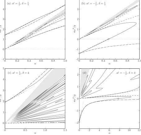
II.2.4. Single mode, arbitrary rotation rate solutions: numerics
In order to obtain results at arbitrary rotation rate we proceed using a hybrid of analytical and numerical methods, whereby evaluation of integrals is carried out using Simpson’s rule. For N = 1, n = 1 we construct the matrix of coefficients ofcjnfrom the linear equations
∂Φ/∂cjn = 0 for j = 1,2. This yields a 2×2 matrix, M, and the zeros of its determinant, corresponding to possible solutions, are calculated numerically and plotted in Fig. 3 forA =±1
2, δ= 1
4,4. The zero rotation rate solutions, as found by Taylor [24], are indicated by white circles on the vertical axes. Selectingn= 1 givesk=k1, the first zero ofJ1, and so we havek≈3.83.
Inertial waves are present as a result of the rotation and it can be seen that these solutions all converge at the origin indicating that as the rotation rate tends to zero these waves are not supported, consistent with their definition. The first pair of inertial wave solutions, corre-sponding to (38) withq= 1, are indicated by dot-dashed lines extending away from the origin. The grayed-out regions contain an infinite number of inertial waves cor-responding to the higher values ofq. Within this region the numerical contouring of|M|= 0 fails and so the re-gion has been grayed-out.
In the stable cases, A = 1
a
ω
2/
g
α (a)A = 1
2,δ= 1 4
0 0.2 0.4 0.6 0.8 1.0
-1 0 1 2 3 4 5
a
ω
2 /
g
α (b)A =−1
2,δ= 1 4
0 0.2 0.4 0.6 0.8 1.0
-2 -1 0 1 2 3 4
a
ω
2/
g
α (c)A =1
2,δ= 4
0 0.5 1.0 1.5
0 1 2 3 4 5
a
ω
2 /
g
α
(d) A =−1
2,δ= 4
0 2 4 6 8 10 12
[image:9.612.87.541.85.521.2]-2 -1 0 1 2
FIG. 3: Solutions of the eigenvalue problem, consistent with the assumptions of§II.1, describing the dispersion relation for Atwood numbersA =±1
2 (stable and unstable respectively),δ= 1
4,4,N = 1,k=k1≈3.83. Solid lines are the exact solution calculated numerically. The long-dashed lines correspond to Chandrasekhar’s solution (34).
(a) Stable: A =1
2,δ= 1
4. The gravity wave solution coincides with theα= 0 axis at the value given by Taylor, indicated by a circle. The asymptotic solution is shown dashed forα <0.5 and continues dotted for larger values.
The first pair of inertial wave solutions (38) corresponding toq= 1 are shown (dot-dashed). The greyed region contains an infinite number of possible inertial wave solutions corresponding to higher values ofq. (b) Unstable:
A =−1
2,δ= 1
4. Onα= 0 the unstable growth is predicted by Taylor’s [24] result. It can be seen that as the rotation rateαincreases, one of theq= 1 inertial wave solutions coalesces with the gravity wave solution. The critical rotation rate is predicted by (43) and is given byαc = 0.49. (c)A =12,δ= 4. With the increase in δwe see
an improvement between the full solution and Chandrasekhar’s solution, giving better agreement than the low rotation rate asymptotics (32). (d)A =−1
2,δ= 4. There is excellent agreement with Chandrasekhar’s solution for
α <5 compared with the low rotation rate asymptotics, but his solution remains in the unstable region asα→ ∞, unlike the full solution. The critical rotation rate,αc= 7.78, follows from (43). As in (b), one of theq= 1 inertial
are shown as the dashed lines extending away from the white circle on the vertical axes. They are shown dashed forα <0.5, after which we anticipate the approximations being less good, as the errors areO(α2), and the solution is thereafter shown as dotted.
In the unstable cases, A =−1
2, shown in Fig. 3b, d, the effect of rotation on the k1 gravity wave at the in-terface is to change the sign of ω2 from negative (un-stable – Rayleigh-Taylor instability) to positive ((un-stable – standing wave solutions). The rotation is able to com-pletely stabilize the mode for α > αc. It can be seen that as the rotation rate is increased the gravity wave solution coalesces with the dominant inertial wave solu-tion. The predicted critical rotation rates areαc ≈0.49 for δ= 1
4 and αc ≈7.78 for δ= 4. It can be seen that for moderate values of α there is significant improve-ment in the agreeimprove-ment between the numerical solution and Chandrasekhar’s [3] solution for the larger value of
[image:10.612.327.562.541.707.2]δ, as expected (see§II.2.1). With the parameters used in Fig. 3b, the asymptotic value ofαc calculated for large
N is within 3.4% of that calculated usingN = 1 modes, as in (43).
It can be shown that as a result of (40 b), the key results of §II.2, (32) and (43), are independent of the Ω2/(1−µ2) term in (27), the only term that has an ex-plicit dependence on the profile z0(r). As the low ro-tation rate approximation (32) and the critical roro-tation rate (43) are independent of this term it follows that the unstable solution branch forωcan be well-approximated by neglecting this term. Indeed, for low to moderate At-wood number (A <
∼ 1 2) then
Φ∝
Z a
0
ω2φˆ2−φˆ1
2
−gA ∂
∂z
ˆ
φ22−φˆ21
z=z0(r)
rdr
(44) is a reasonable approximation to (27), with approximate O(A2) error. The calculated critical rotation rate for
the example considered in Fig. 3b using (44), as opposed to (27), isαc = 0.45 compared toαc= 0.49, an error of approximately 7.8%.
II.3. Non-axisymmetric instability,m6= 0
We now consider the more general case which includes non-axisymmetric modes. Here, the right hand side of (29) can be non-zero, and soω ∈C, giving the possibil-ity of both growth and precession of the instabilpossibil-ity. As
ω ∈ C it follows that k =k(Ω, ω)∈ C in general. The fact that kcannot be determined a priori for the whole solution space increases the difficulty of calculating so-lutions for the non-axisymmetric cases compared to the axisymmetric cases.
II.3.1. Single mode, low rotation rate, gravity wave solutions: asymptotics
To find the corresponding low rotation rate asymp-totics as in§II.2 we expand bothω andkin terms ofα. It follows from (29) forω∼ω0+ω1α1/2+ω2α+. . .that
k k0
∼1 + 2m
k2 0−m2
αg aω2
0
1/2
− 2m
k2 0−m2
"
aω2 1
g
1/2
+m k 2 0+m2
(k2 0−m2)
2
#
αg aω2
0
+O(α3/2), (45)
wherek0∈Rsatisfies
k0Jm+1(k0) =mJm(k0). (46)
(Note that again there are a countable number of solu-tionsk0n but for clarity we will use the notationk0 and understand that it may not be the first zero of (46).) Substituting in and following a similar procedure to that in§II.2, the first two terms forω satisfy
aω2 0
g =Ak0tanh(k0δ), (47a)
ra
gω1= m k2
0−m2
[1 + 2k0δcsch (2k0δ)]. (47b)
The leading order termω0is unchanged from (32), noting the change in definition ofk0. Theω1term is not present in (32), as a result ofm = 0 in the axisymmetric case. However we note thatω1 ∈Rand so this term can play no role in the growth or suppression of interfacial waves; it is merely contributing a modification to the precession velocity. We also note thatω1is independent ofA and is therefore exactly the same as the first correction term found by Miles [13, eq. (5.5)].
For comparison with the second term on the right hand side of (32) we now calculatea(2ω0ω2+ω12)/g and find it to be
2
(
1− 2m 2k2
0 (k2
0−m2)
3+ 2k0δcsch (2k0δ)
×
1− m
2 (k2
0−m2)2
k2 0+m2
k2 0−m2
+ 2k0δcoth (2k0δ)
−1 8k
2
0A2sech (k0δ)2
1 + 4
k2 0−m2
×
m2 k2 0
cosh (k0δ)2−k02G(m, k0)
, (48)
where we use (40 a–c) and define
G(m, k) =
Z 1
0
Jm(kx)2 Jm(k)2 x
3dx. (49)
Providedk0is a solution of (46) then in the limitm→0,
m= 0 term in (32) from (48). The associated eigenvector with the solution described by (47) and (48) is
c=
1,−1−k0
2 coth (k0δ)
×
1 + 4
k2 0−m2
m2
k2 0
−k20G(m, k0)
α+O(α2)
,
(50)
and we note that therefore to leading order the solution in the lower layer is growing and precessing in the opposite direction to the fluid in the upper layer, as might have been anticipated.
It follows from (48) that ω2 ∈ C if ω0 ∈ C and so may contribute to both precession and growth/decay. Whether the growth rate of a wave mode is reduced or increased by a small amount of rotation, compared to its growth in a non-rotating system, is controlled by (48) too, sinceω1∈R.
II.3.2. Single mode, low rotation rate, inertial wave solutions: asymptotics
As with the axisymmetric case, forω2to have a leading order contribution of O(α) we require (36) and hence (37) to be satisfied. Writingω∼ω1α1/2+ω2α+. . . and
k∼k0+k1α1/2+k2α+. . .we have that
ω2 1a
g =
4 1 + [2k0δq]2
for δq ≡ δ
qπ, and q∈N.
(51) The leading order balance of (29) is therefore
Jm+1(k0) =
m k0
1 + 2
ω1
Jm(k0). (52)
Combining (51) and (52) we have that for a givenm6= 0 andδq,k0 must satisfy
1 + [2k0δq]2=
1−k0
m
Jm+1(k0) Jm(k0)
2
. (53)
The solutions fall into two categories according as to whetherqis odd or even, as before. Forqodd
ω2a
g ∼
4α
1 + [2k0δq]2
×
1∓α[2k0δq] 2 2δ 1 + 4
δq2m2−G(m, k0)
×
"
1 + 4δq2m2
1 + [2k0δq]2− 8mδ2
q
ω1
#−1
. (54)
The expression forq-even is lengthy and so here we note only the solutions for extreme values ofδ. Specifically, if
qis even andm6= 0, then forδ≪1
ω2a
g ∼4α
(
1±2δ 2 qα
δ k
2
0[1−4G(m, k0)] + 4m
+O(α2)
)
, (55)
and forδ≫1
ω2a
g ∼4α
1
[2k0δq]2 ±α
δ m δqk30
+O(α2)
. (56)
A further, higher order, solution exists, providedm6= 0, fork∼k0+O(α) whereJm(k0) = 0 and
ω2a
g ∼
2m
k2 0δ
2
α3
(
1− α 2δ
"
4G+(m, k0)
−1 + 4
k2 0
1±A2
#
+O(α2)
)
, (57)
where
G+(m, k) =
Z 1
0 J2
m(kx) J2
m+1(kx)
x3dx. (58)
II.3.3. Single mode, critical rotation rate for stabilization
In§II.2.3 it was shown that for δ <∞ there exists a critical rotation rate, Ωc, above which an axisymmetric wave mode can be stabilized for a given unstable Atwood number. Here we show that such a critical rotation rate does not exist in the casem6= 0.
Form6= 0 and Ω∼Ω01 + (Ω1/Ω0)ω+O(ω2), (29) implies that
k k0
∼1− ω
2mΩ0
+O(ω2), where Jm(k0) = 0, (59)
noting thatm6= 0 changes the definition ofk0 from the axisymmetric definitionJm+1(k0) = 0, to Jm(k0) = 0. The eigenvalue equation for Ω becomes
1−A2
A2
a2mΩ0Jm+12 (k0) 2
ω2+O ω3
= 0. (60)
It can be seen that there is no non-zero critical rotation rate, Ω0, that can force the leading order term in (60) to be zero. Therefore, unlike the axisymmetricm= 0 case, there does not exist a critical rotation rate that can be used to stabilize a given wave mode. However, a given wave mode may still be suppressed (or indeed excited) by rotation, but a change of stability cannot occur.
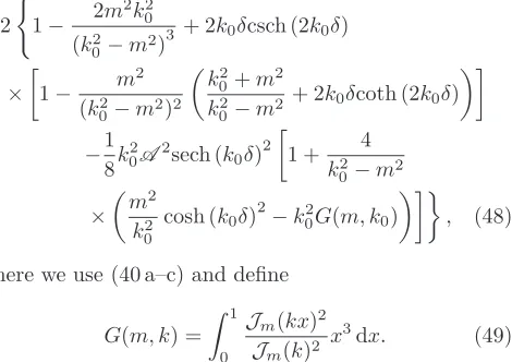
II.3.4. Single mode, arbitrary rotation rate solutions: numerics
The solutions of the eigenvalue problem are calculated numerically forN = 1,n= 1,δ= 14,A =−1
ℑ
(
ω
)
α
ℜ(ω)
(a)
0
1 0
1 0
-0.7
m= 1
ℜ
(
a
ω
2 /
g
)
−
ℑ
(
a
ω
2 /
g
)
α
(b) m= 1
0 0.2 0.4 0.6 0.8 1.0
-0.5 0 0.5
ℜ
(
a
ω
2/
g
)
−
ℑ
(
a
ω
2/
g
)
α
(c) m= 2
0 0.2 0.4 0.6 0.8 1.0
-1.0 0 0.5
ℜ
(
a
ω
2 /
g
)
−
ℑ
(
a
ω
2 /
g
)
α
(d) m= 3
0 0.2 0.4 0.6 0.8 1.0
-2.0 0 1.0
FIG. 4: (a) The constructed solution of|M|= 0 forω∈CandA =−1
2,δ= 1
4,N = 1,n= 1,m= 1 (solid lines). (b)–(d) Are projections of the solution squared, for comparison with Fig. 3b. Bold solutions have non-zero imaginary component. It can be seen that unstable wave modes are not stabilized by increasing the rotation rate,
but are suppressed initially. Asymptotic gravity wave approximations (47), (48) to the solution are shown dot-dashed. (Inertial wave solutions not shown.)
1,2,3 (see Fig. 3b for comparison with the axisymmetric case,m= 0).
The numerical solution was calculated by evaluating the determinant ofM for a givenα over a planeω ∈ C (numerical integration was carried out using Simpson’s rule). The zeros of the real part of|M| were contoured and intersections with the zero contour of the imagi-nary part of |M| were found. The solution was con-structed by then allowingαto vary over the range [0, αT] (see Fig. 4a). Figs 4b–d are projections of the three-dimensional solution to allow comparison with Fig. 3b. The positive vertical axis shows a projection ofℜ(ω)2a/g
[image:12.612.80.544.56.500.2]ℑ
(
ω
)
α
ℜ(ω)
(a)
0
2 0
2 0
-2
ℜ
(
a
ω
2/
g
)
−
ℑ
(
a
ω
2/
g
)
α
(b) m= 2
N = 2
0 0.5 1.0 1.5 2.0
[image:13.612.69.290.70.497.2]-4 0 4
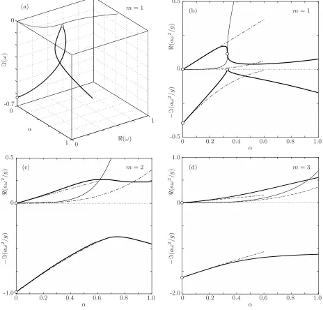
FIG. 5: Gravity wave solutions of|M|= 0 forA =−1
2,
δ= 14,m= 2 forN = 2 andn= 1,2, i.e.,k01≈3.054 andk02≈6.706. Bold solutions have non-zero
imaginary component. (a) Three-dimensional representation of the solution: the most unstable branches cross atα≈1.505, whereω1≈1.514−1.313i
andω2≈0.189−1.313i indicated by circles. (b) The projected solutions for comparison with Fig. 3b. AlthoughαT = 1, theαaxis has been extended to show
the possibility of rotation causing some modes to become more unstable than others.
II.3.5. Multiple mode, arbitrary rotation rate solutions
Fig. 5 shows the possible wavemodes for A = −1
2,
δ = 14, m = 2, N = 2, and n = 1,2. As the rotation rate is increased the unstable gravity wave modes are seen to be suppressed, though the suppression is greater
for the more unstablen= 2 mode. The plot shows that suppressing a higher wavemode to such an extent that it becomes more stable than a lower wavemode is possi-ble since the solution’s projections cross (atα ≈1.505, ℑ(ω) ≈ −1.313, shown as circles, though in this case the crossing occurs forα > αT where the solution is not strictly valid). Comparing Fig. 4c with Fig. 5b, it can be seen that the addition of a single extra mode significantly increases the number of possible modes of behavior.
II.4. Summary of key results
In§II.1 the approach developed by Miles [13] to model surface waves on a rotating body of water was gener-alised to the two-layer case, allowing for either a stable (positive Atwood number) or an unstable (negative At-wood number) initial stratification. The dispersion rela-tion for axisymmetric perturbarela-tions at low rotarela-tion rates was derived in§II.2, (32), which shows that gravitation-ally unstable perturbations may be made less unstable by rotating the system. This suggests that at least par-tial suppression of the Rayleigh-Taylor instability may be achieved through rotation of the system, though we note that the dispersion relation (32) is only valid in the low-rotation rate limitaΩ2/g≪1. In§II.2.3 an exact re-sult, (43), was found for the critical rotation rate required to completely stabilise an otherwise gravitationally un-stable axisymmetric wave mode. This critical rotation rate depends on the aspect ratio of the system which is the reason an exchange of stability was not found in the model of Chandrasekhar [3]. The critical rotation rate in (43) indicates that a rotation rateαc= 12δis required to stabilise all axisymmetric wave modes, but the model solutions (28) are invalid forα >4δ.
In §II.3 the dispersion relation for asymmetric wave modes was derived (45)–(49). This dispersion relation includes axisymmetric perturbations, m = 0, as a spe-cial case. In the asymmetric case, m6= 0, it was shown that the wavenumber cannot be determineda priori, it depends on both the rotation rate, Ω, and the mode fre-quency,ω. The dispersion relation reveals, as might be anticipated, that the mode frequency contains both real and imaginary parts in general. Hence, the developing instability is characterised by both a growth and a pre-cession of a given wave mode. It was also shown,§II.3.3, that a general critical rotation rate to stabilise an asym-metric mode does not exist, unlike the axisymasym-metric case.
2(gd)1/2/a, then (43) indicates that the mode may be stabilised indefinitely. Rotation was also seen in some cases to be able to slow the growth of asymmetric modes. We can understand our observations in the following qualitative manner: a rotating fluid is known to organise itself into coherent vertical structures aligned with the axis of rotation, so-called ‘Taylor columns’ [23], whereas a perturbation to an unstable two-layer density strati-fication will lead to baroclinic generation of vorticity at the interface, tending to break-up any vertical structures. Hence the system under investigation undergoes compe-tition between the stabilising effect of the rotation, that is organising the flow into vertical structures and prevent-ing the two fluid layers passprevent-ing each other, and the
desta-bilising effect of the denser fluid overlying the lighter fluid that generates an overturning motion at the interface. With increased rotation rate the ability of the fluid layers to move radially, with opposite sense to each other, in or-der to rearrange themselves into a more stable configura-tion, is increasingly prohibited by the Taylor-Proudman theorem [see 15, 22]. The radial movement is therefore reduced and the observed structures that materialize as the instability develops are smaller in scale.
MMS acknowledges funding from EPSRC under grant number EP/K5035-4X/1, RJAH acknowledges support from EPSRC Fellowship EP/I004599/1. We thank L. Eaves, P. Linden, E. Hall and M. Swift for useful dis-cussions.
[1] K. A. Baldwin, M. M. Scase, and R. J. A. Hill, The inhibition of the Rayleigh-Taylor instability by rotation. Sci. Rep.5, 11706 (2015).
[2] G. F. Carnevale, P. Orlandi, and Y. Zhou, Rotational suppression of Rayleigh-Taylor instability. J. Fluid Mech.
457, 181 (2002).
[3] S. Chandrasekhar, Hydrodynamic and Hydromagnetic Stability. (New York: Dover, 1961.)
[4] B. A. Finlayson,The Method of Weighted Residuals and Variational Principles(Academic Press, 1972.)
[5] J. R. Freeman, M. J. Clauser, and S. L. Thompson, Rayleigh-Taylor instabilities in inertial confinement fu-sion targets. Nuclear Fufu-sion17(2), 223 (1977).
[6] D. Fultz, An experimental view of some atmospheric and oceanic behavioral problems. Trans. N. Y. Acad. Sci.24, 421 (1962).
[7] R. W. Hart, Generalized scalar potentials for linearized three-dimensional flows with vorticity. Phys. Fluids
24(8), 1418 (1981).
[8] H. Lamb, 1932Hydrodynamics(6th edn. Cambridge Uni-versity Press, 1932).
[9] D. J. Lewis, The instability of fluid surfaces when ac-celerated in a direction perpendicular to their planes. II. Proc. Roy. Soc. A202, 81 (1950).
[10] M. J. Lighthill,Waves in Fluids(Cambridge University Press, 1978).
[11] J. Lindl, Development of the indirect-drive approach to inertial confinement fusion and the target physics basis for ignition and gain. Phys. Plasmas2(11), 3933 (1995). [12] J. W. Miles, Free surface oscillations in a rotating fluid.
Phys. Fluids2(3), 297 (1959).
[13] J. W. Miles, Free-surface oscillations in a slowly rotating fluid.J. Fluid Mech.18(2), 187 (1964).
[14] H. Poincar´e, Sur l’´equilibre d’une masse fluide anim´ee
d’un mouvement de rotation. Acta Math. 7 (1), 259 (1885).
[15] J. Proudman, On the motion of solids in a fluid possessing vorticity. Proc. Roy. Soc. Lond. A92(642), 408 (1916). [16] Lord Rayleigh, Investigation of the character of the
equi-librium of an incompressible heavy fluid of variable den-sity. Proc. Roy. Math. Soc.14, 170 (1883).
[17] M. M. Scase and S. B. Dalziel, Internal wave fields and drag generated by a translating body in a stratified fluid. J. Fluid Mech.498, 289 (2004).
[18] M. M. Scase and S. B. Dalziel, Internal wave fields gen-erated by a translating body in a stratified fluid: an ex-perimental comparison. J. Fluid Mech.564, 305 (2006). [19] M. M. Scase, K. A. Baldwin and R. J. A. Hill, Magnetically-induced Rotating Rayleigh-Taylor Instabil-ity. J. Vis. Expt.In Press(2016).
[20] P. K. Sharma, R. P. Prajapati, and R. K. Chhajlani, Ef-fect of surface tension and rotation on Rayleigh-Taylor instability of two superposed fluids with suspended par-ticles. ACTA Physica Polonica A118(4), 576 (2010). [21] J. J. Tao, X. T. He, W. H. Ye, and F. H. Busse,
Nonlin-ear Rayleigh-Taylor instability of rotating inviscid fluids. Phys. Rev. E87, 013001 (2013).
[22] G. I. Taylor, Motion of solids in fluids when the flow is not irrotational. Proc. Roy. Soc. Lond. A 93 (648), 99 (1917).
[23] G. I. Taylor, Experiments on the motion of solid bodies in rotating fluids. Proc. Roy. Soc. Lond. A104, 213 (1923). [24] G. I. Taylor, The instability of fluid surfaces when ac-celerated in a direction perpendicular to their planes. I. Proc. Roy. Soc. A201, 192 (1950).
[25] C.-Y. Wang, and R. A. Chevalier, Instabilities in clump-ing and type 1a supernova remnants. Astrophys. J.
![FIG. 2: Two layers of incompressible fluid of density ρbeing accelerated [see 24] at a ratez1and ρ2 occupy a cylindrical tank of radius a that is g1](https://thumb-us.123doks.com/thumbv2/123dok_us/8585015.370266/3.612.64.288.61.310/layers-incompressible-uid-density-rbeing-accelerated-occupy-cylindrical.webp)