Wave Interaction with Defects in Pressurized
Composite Structures
R.K. Apalowo, D. Chronopoulos and V. Thierry
Abstract—A wave finite element (WFE) and finite element (FE) based computational method is presented by which the dispersion properties as well as the wave interaction coefficients for one-dimensional structural system can be predicted. The structural system is discretized as a system comprising a number of waveguides connected by a coupling joint. Uniform nodes are ensured at the interfaces of the coupling element with each waveguide. Then, equilibrium and continuity conditions are enforced at the interfaces. Wave propagation properties of each waveguide are calculated using the WFE method and the coupling element is modelled using the FE method. The scattering of waves through the coupling element, on which damage is modelled, is determined by coupling the FE and WFE models. Furthermore, the central aim is to evaluate the effect of pressurization on the wave dispersion and scattering characteristics of the prestressed structural system compared to that which is not prestressed. Numerical case studies are exhibited for two waveguides coupled through a coupling joint.
Keywords—Finite Element, Prestressed Structures, Wave Finite Element, Wave Propagation Properties, Wave Scattering Coeffi-cients.
I. INTRODUCTION
Composite structures are increasingly used in modern aerospace and automobile industries due to their well-known benefits. However, they exhibit a wide range of structural failure modes for which the structures has to be frequently and thoroughly inspected in order to ensure continuous structural integrity. Aeronautical industry lost approximately 27% of an average modern aircraft’s lifecycle cost [1] on inspection and repair.
Implementing a suitable modelling technique is as important as selecting an appropriate NDE method for SHM. The Finite Element (FE) method [2] is one of the most common ones employed to analyse the dynamic behaviour of structures. The Wave Finite Element (WFE) method was introduced in [3] to facilitate the post-processing of the eigenvalue problem solutions. The method has been successfully implemented in 1-D [3], [4] and 2-D [5], [6] wave propagation analyses. The method has recently found applications in predicting the vibroacoustic and dynamic performance of composite panels and shells [7], [5], [8], [9] , with pressurized shells [10], [11], cylindrical pipes [12] and complex periodic structures [13], [14], [15] being investigated. The variability of acoustic transmission through layered structures [16], [17], as well as wave steering effects in anisotropic composites [18] have been modelled through the same methodology. The same FE based approach was employed to compute the reflection and transmission coefficients of waves impinging on linear joints
in [4], point and finite joints [19] as well as curved [20] and stiffened [21] panels .
In this work, the effect of structural prestressing on wave propagation properties and wave interaction characteristics of composite structure is presented. Wave propagation properties of the prestressed structure is computed through one dimen-sional WFE approach. The structure can be of arbitrary com-plexity, layering and material characteristics as FE modelling is employed. The structure is discretised as system of two or more waveguides connected together by a joint (otherwise known as the coupling element). The WFE calculated wave propagation properties within the structural waveguides is coupled to the FE modelling of the coupling element. Both the non prestressed and prestressed scenarios are considered. The paper is organised as follows: Section II presents the formulation of the WFE method for predicting the wave propagation properties. Section III presents wave interaction with structural damage and the computation of the interac-tion characteristics. Secinterac-tion IV presents example case studies along with the numerical results. Finally, conclusions on the presented work are presented in Section V.
II. WAVE PROPAGATION IN A PRESTRESSED STRUCTURE BY THEWFEMETHOD
A. Prestressing
Internal pressurisation of the structure is considered. The stress stiffening effect as a result of the pressurisation is accounted for by augmenting a prestress stiffness matrix,Kp,
to the conventional stiffness matrix,K0, of the system.Kpis
dependent on the geometry, displacement field and the state of stress of the structural element [22]. For a 3-D element, which is considered in this work, the pre-stress stiffness matrix is given as [23]
Kp= Z Z Z
S⊤gSmSgdx dy dz (1)
whereSg is the shape function derivative matrix, Sm is the Cauchy stress tensor and[•]⊤ is a transpose. Hence, the total
stiffness matrix of the prestressed system is given as
K=K0+Kp (2)
B. Wave propagation in arbitrary layered structure by a WFE method
ܮ௫
ࡸ
ࡾ
[image:2.595.347.529.101.232.2]ࡵ
Fig. 1. WFE modelled waveguide with the left and right side nodesqL,qR
bullet marked. The range of interior nodesqIalso illustrated
problem is solved using the WFE method (coupling FE to the periodic structure theory) as in [3].
The frequency dependent DSM can be partitioned with regards to the left L, right R and internal I DoFs of the periodic segment as
DLL DLI DLR
DIL DII DIR
DRL DRI DRR qL qI qR = fL 0 fR (3)
withqandfthe displacement and forcing vectors respectively. Eq. (3) is condensed using a Guyan-type condensation tech-nique. Assuming no external forces are applied to the segment, then the displacement continuity and equilibrium of forces equations at the interface of two consecutive periodic segments are given as
qsR=q s+1
L f
s R=−f
s+1
L (4)
The transfer matrix, T, which relates the displacement and force vectors of the left and right sides of the periodic segments is obtained as
qsL+1 fLs+1
=T qs L fs L (5)
where the expression of the symplectic transfer matrix is defined as
T =
D11 D12 D21 D22
(6)
where
D11=−(DLR−DLIDII−1DIR)−1(DLL−DLID−1 II DIL) D12= (DLR−DLID−II1DIR)−1
D21= (−DRL+DRID−II1DIL) + (DRR+DRID−II1DIR) (DLR−DLID−1II DIR)−1(DLL−DLID−1
II DIL) D22=−(DRR+DRID−II1DIR)(DLR−DLID−II1DIR)−1
(7)
WFE model
FE model
Fig. 2. Periodic structure comprising of two waveguides and a coupling element
Constant of propagation,λ=e−ikLx
, of the waves relates the left and right hands nodal values to each other as
qsR=λqs L f
s R=−λf
s
L (8)
then the eigenproblem relation for the periodic segment can be expressed as
λ
q⊤L fL⊤ ⊤=T q⊤L fL⊤ ⊤ (9)
whose eigenvalues λω and eigenvectors φω = λ
φq φf
ω
solution sets provide a comprehensive description of the propagation constants and the wave mode shapes for each of the elastic waves propagating in the structural waveguide at a specified angular frequency.
III. WAVE INTERACTION WITH STRUCTURAL DAMAGE
The wave interaction coefficients of coupling joint in the prestressed waveguide structure is modelled using a hybrid WFE/FE approach. A number of waveguides (for instance two as in Fig. (2) are connected through a coupling joint. The coupling joint is fully FE described and can contain damage, geometry or material inconsistencies etc.
Once the propagation constants of each prestressed waveg-uide have been sought as presented in Section II, each wavemode w with w ∈ [1· · · W] for waveguide n with
n∈[1· · · N]in the system can be grouped as
Φ+n,q = [φ+q,1 · · · φ+q,W] Φ+n,f = [φ+f,1· · · φ+f,W]
Φ−
n,q = [φ −
q,1 · · · φ
−
q,W] Φ
−
n,f = [φ −
f,1· · · φ
−
f,W]
(10) The wavemodes of the entire system can be computed at each specified angular frequency and be grouped as
Φ+q =
Φ+1,q 0 · · · 0 0 Φ+2,q · · · 0
· · · ·
0 0 · · · Φ+N,q
[image:2.595.92.262.103.280.2]with similar expressions for Φf, Φq and Φf . The rotation matrix Rn transforms the DoFs of each waveguide from the local to the global coordinates of the system as
Φg,q+=RΦ+q (12)
with similar expressions forΦg,f +,Φg,− q andΦ
g,−
f . g denotes
the global coordinates index and R represents the rotation matrices of the system’s waveguides, grouped in a block diagonal matrix.
Waves of amplitudes an+ are impinging on the coupling element from the nth waveguide. These give rise to reflected waves of amplitudes an− with an− = cn,nan+ in the n
waveguide and transmitted waves of amplitudes ak− with ak−=ck,nan+ in thekth waveguide, and vice versa. Hence,
the incident waves amplitudes can be related to the amplitudes of the scattered waves (reflection and transmission) as
a−=Sa+ (13)
with a+[WN×1] the vector containing the amplitudes of the incident waves (on the coupling joint) anda−[WN×1]the vec-tor containing the amplitudes of the reflected and transmitted waves.
The frequency dependent DSM of the FE modelled coupling joint can be partitioned with regards to the interface i and non-interfacesnnodes of the coupling joint with the system’s waveguides as
Dii Din Dni Dnn
qJ i qJ n
=
fJ
i 0
(14)
where J is the coupling joint index. using a Guyan-type condensation for the non-interface DoF, the problem can be expressed as
DJqJi =fiJ (15)
with
DJ=Dii−DinD−nn1Dni (16)
A transformation can be defined for the motion in the waveguides between the physical domain, where the motion is described in terms of q(t)andf(t) and the wave domain, where the motion is described in terms of waves of amplitudes
a+ anda− travelling in the positive and negative directions respectively as
q(t) =Φ+qa++Φ
− qa− f(t) =Φ+f a++Φ
− f a−
(17)
Expressing the continuity and equilibrium equations of the coupling joint in the wave domain, then the scattering coefficients matrix of the joint can be expressed as
S=−[Φg,f −−DJΦg,q−]−1[Φg,f +−DJΦg,q+] (18)
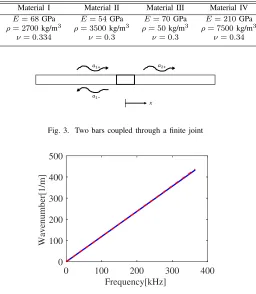
TABLE I
MECHANICAL PROPERTIES OF MODELS MATERIALS
Material I Material II Material III Material IV
E= 68GPa E= 54GPa E= 70GPa E= 210GPa ρ= 2700kg/m3
ρ= 3500kg/m3
ρ= 50kg/m3
ρ= 7500kg/m3
ν= 0.334 ν= 0.3 ν= 0.3 ν= 0.34
ݔ ܽ
ଵା ܽ
ଶା
ܽ
[image:3.595.312.568.127.421.2]ଵି
Fig. 3. Two bars coupled through a finite joint
Frequency [kHz]
0 100 200 300 400
Wavenumber [1/m]
0 100 200 300 400 500
Fig. 4. Dispersion curves for the bar: analytical(-), WFE(- -)
IV. NUMERICAL CASE STUDIES
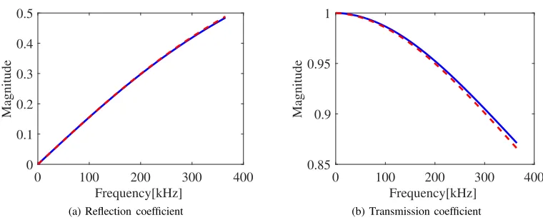
Three numerical case studies are presented. The first, two collinear bars connected through another bar of a different material characteristics. An analytical solutions exists for the dispersion relation and wave scattering coefficients of the problem. The second and third case studies are monolithic and sandwiched laminates respectively. The laminates are considered under non-pressurised and pressurised scenarios. The mechanical properties of the materials used in the models are given in Table I.
A. Two Collinear bars coupled through a finite bar
Two similar and collinear long bars undergoing longitudinal vibration is considered. A finite beam of a different material properties is sandwiched between them as shown in Fig. (3). Cross-sectional areas A1 = A2 = AJ = 0.003m2, lengths L1 = L2 = 0.2m andL = 0.003m. Material I (Table I) is used for both bars and Material IV for the coupling joint.
Frequency [kHz]
0 100 200 300 400
Magnitude
0 0.1 0.2 0.3 0.4 0.5
(a) Reflection coefficient
Frequency [kHz]
0 100 200 300 400
Magnitude
0.85 0.9 0.95 1
[image:4.595.116.496.107.261.2](b) Transmission coefficient
Fig. 5. Wave interaction coefficients for a finite joint connecting two bars: analytical(-), WFE-FE(- -)
B. Prestressed monolithic laminate
Two collinear monolithic laminates connected by a coupling joint (another monolithic laminate) of the same cross-section (0.01m×0.005m) as the two laminates is considered. The laminates are modelled using Material I (Table I). An illustra-tion of the WFE model of each waveguide and the FE model of the coupling joint is presented in Fig. (2). The length of the coupling joint is0.004mwhile that of each waveguide is arbitrary, as only one periodic segment is needed for the WFE model. Each laminate in the system is prestressed with internal pressurisation of upto 1 GPa. Surface breaking crack of depth 20% of the total depth of the coupling joint. The damage is located at the mid length of the coupling joint.
The dispersion relation at 100 MPa pressurisation is quite close to that of the non-pressurised system, unlike the high pressurised system whose dispersion relation is comparatively different. This indicates that the applied pressurisation can only have significant effect on the waves dispersion properties if its magnitude is in the range of the stiffness property of the structure.
The waves reflection coefficients of each of the propagating waves are presented Fig. (7). The results are compared for the non-pressurised and pressurised systems in each case. Gen-erally, notable differences are observed in the wave reflection characteristics of the pressurised systems compared to the non-pressurised systems especially in the torsional wave results. Consequently, the magnitude of wave interaction coefficients in the pressurised system can be used to detect micro defects which may not be easily detected without the presence of pressurisation.
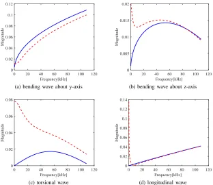
C. Prestressed composite laminate
Two collinear composite laminates connected by a coupling joint (another composite laminate) of the same cross-section is considered. Each periodic segment of the asymmetric compos-ite laminate consists of a core (honeycomb foam) sandwiched between two carbon epoxy facesheet layers. The core is modelled using Material III (Table I) while the facesheet is modelled using Material II. The length of the coupling joint
is0.004m. The upper facesheet, lower facesheet and the core of the periodic segment are0.002m,0.001mand0.01mdeep respectively.0.002mdepth surface breaking crack is modelled on the coupling joint. The damage is located at the mid length of the joint.
The dispersion curves, of each propagating wave, for the non-pressurised and pressurised composite laminates are pre-sented in Fig. 8. Except for the longitudinal wave with quite little difference, the wavenumber of the propagating waves in the pressurised system is significantly different compared to that of the non-pressurised system, especially within the frequency range of [0.2 kHz, 20 kHz].
Fig. (9) presents the results, of the reflection coefficient magnitude of each propagating waves. Comparing the results of the non-pressurised system with that of the pressurised system, the reflection coefficient magnitude of the y-axis bending and the torsional waves is significantly different especially within frequency [0.2 kHz, 20 kHz]. The torsional wave shows highest level of difference, in the reflection coefficient magnitude, due to the pressurisation. The difference in the wave interaction coefficient magnitude of the pressurised composite laminate and the non-pressurised one can be said to be as a result of an increase in the strain energy of the honeycomb core due to the internal pressurisation.
V. CONCLUDING REMARKS
The effect of prestressing on the wave propagation proper-ties and the wave interaction coefficients of laminated struc-tural systems is evaluated in this work. A comprehensive FE based computational scheme is presented for quantifying wave interaction effects with damage within structures of arbitrary layering and geometric complexities. The structural system is modelled by hybrid coupling of the WFE modelling of two waveguides, and a FE model of a coupling element, through which waves propagate from one waveguide to the other. The presented methodology is evaluated by comparing its results with the theoretically obtained results for the case of two bars connected by a finite coupling joint.
Frequency [kHz]
0 20 40 60 80 100 120
Wavenumber [1/m]
0 100 200 300
(a) bending wave about y-axis
Frequency [kHz]
0 20 40 60 80 100 120
Wavenumber [1/m]
0 50 100 150 200 250
(b) bending wave about z-axis
Frequency [kHz]
0 20 40 60 80 100 120
Wavenumber [1/m]
0 50 100 150 200 250 300
(c) torsional wave
Frequency [kHz]
0 20 40 60 80 100 120
Wavenumber [1/m]
0 20 40 60 80 100 120 140
[image:5.595.150.463.123.399.2](d) longitudinal wave
Fig. 6. Dispersion curves for the non-pressurised (-), 100 MPa (- -) and 1 GPa (-◦) pressurised monolithic laminate
Frequency [kHz]
0 20 40 60 80 100 120
Magnitude
0 0.02 0.04 0.06 0.08 0.1 0.12
(a) bending wave about y-axis
Frequency [kHz]
0 20 40 60 80 100 120
Magnitude
0 0.005 0.01 0.015 0.02
(b) bending wave about z-axis
Frequency [kHz]
0 20 40 60 80 100 120
Magnitude
0 0.02 0.04 0.06 0.08
(c) torsional wave
Frequency [kHz]
0 20 40 60 80 100 120
Magnitude
0 0.02 0.04 0.06 0.08 0.1 0.12 0.14
(d) longitudinal wave
[image:5.595.151.463.465.735.2]Frequency [kHz]
0 20 40 60 80 100 120
Wavenumber [1/m]
0 50 100 150 200 250 300 350
(a) bending wave about y-axis
Frequency [kHz]
0 20 40 60 80 100 120
Wavenumber [1/m]
0 50 100 150 200
(b) bending wave about z-axis
Frequency [kHz]
0 20 40 60 80 100 120
Wavenumber [1/m]
0 50 100 150 200 250
(c) torsional wave
Frequency [kHz]
0 20 40 60 80 100 120
Wavenumber [1/m]
0 20 40 60 80 100
[image:6.595.150.463.124.399.2](d) longitudinal wave
Fig. 8. Dispersion curves for the non-pressurised (-) and 1 GPa pressurised (- -) composite laminates
Frequency [kHz]
0 20 40 60 80 100 120
Magnitude
0 0.02 0.04 0.06 0.08
(a) bending wave about y-axis
Frequency [kHz]
0 20 40 60 80 100 120
Magnitude
0 0.05 0.1 0.15 0.2
(b) bending wave about z-axis
Frequency [kHz]
0 20 40 60 80 100 120
Magnitude
0 0.01 0.02 0.03 0.04 0.05 0.06 0.07
(c) torsional wave
Frequency [kHz]
0 20 40 60 80 100 120
Magnitude
0 0.05 0.1 0.15 0.2 0.25
(d) longitudinal wave
[image:6.595.151.464.463.734.2]coefficients. Significant differences are observed, for the waves dispersion relation and wave interaction results, between the pressurised and non-pressurised structural systems. This is observed to be more notable if the applied pressurisation is high enough mainly in the range of the structure’s stiffness magnitude.
REFERENCES
[1] S. Kessler, S. Spearing, and C. Soutis, “Damage detection in composite materials using lamb wave methods,”Smart Materials and Structures, vol. 11, pp. 269–278, 2002.
[2] O. C. Zienkiewicz and R. L. Taylor,The finite element method: Solid mechanics. Butterworth-heinemann, 2000, vol. 2.
[3] B. R. Mace, D. Duhamel, M. J. Brennan, and L. Hinke, “Finite element prediction of wave motion in structural waveguides,”The Journal of the Acoustical Society of America, vol. 117, no. 5, pp. 2835–2843, 2005. [4] J.-M. Mencik and M. Ichchou, “Multi-mode propagation and diffusion
in structures through finite elements,”European Journal of Mechanics-A/Solids, vol. 24, no. 5, pp. 877–898, 2005.
[5] D. Chronopoulos, B. Troclet, O. Bareille, and M. Ichchou, “Modeling the response of composite panels by a dynamic stiffness approach,” Composite Structures, vol. 96, pp. 111–120, 2013.
[6] E. Manconi and B. Mace, “Modelling wave propagation in two-dimensional structures using a wave/finite element technique,” ISVR Technical Memorandum, 2007.
[7] D. Chronopoulos, B. Troclet, M. Ichchou, and J. Laine, “A unified approach for the broadband vibroacoustic response of composite shells,” Composites Part B: Engineering, vol. 43, no. 4, pp. 1837–1846, 2012. [8] D. Chronopoulos, M. Ichchou, B. Troclet, and O. Bareille, “Predicting the broadband response of a layered cone-cylinder-cone shell,” Compos-ite Structures, vol. 107, no. 1, pp. 149–159, 2014.
[9] ——, “Computing the broadband vibroacoustic response of arbitrarily thick layered panels by a wave finite element approach,” Applied Acoustics, vol. 77, pp. 89–98, 2014.
[10] V. Polenta, S. Garvey, D. Chronopoulos, A. Long, and H. Morvan, “Optimal internal pressurisation of cylindrical shells for maximising their critical bending load,”Thin-Walled Structures, vol. 87, pp. 133– 138, 2015.
[11] T. Ampatzidis and D. Chronopoulos, “Acoustic transmission properties of pressurised and pre-stressed composite structures,”Composite Struc-tures, vol. 152, pp. 900–912, 2016.
[12] W. Zhou, M. Ichchou, and J. Mencik, “Analysis of wave propagation in cylindrical pipes with local inhomogeneities,”Journal of Sound and Vibration, vol. 319, no. 1, pp. 335–354, 2009.
[13] I. Antoniadis, D. Chronopoulos, V. Spitas, and D. Koulocheris, “Hyper-damping properties of a stiff and stable linear oscillator with a negative stiffness element,”Journal of Sound and Vibration, vol. 346, no. 1, pp. 37–52, 2015.
[14] D. Chronopoulos, M. Collet, and M. Ichchou, “Damping enhancement of composite panels by inclusion of shunted piezoelectric patches: A wave-based modelling approach,”Materials, vol. 8, no. 2, pp. 815–828, 2015.
[15] D. Chronopoulos, I. Antoniadis, M. Collet, and M. Ichchou, “Enhance-ment of wave damping within metamaterials having embedded negative stiffness inclusions,”Wave Motion, vol. 58, pp. 165–179, 2015. [16] D. Chronopoulos, “Design optimization of composite structures
oper-ating in acoustic environments,”Journal of Sound and Vibration, vol. 355, pp. 322–344, 2015.
[17] M. Ben-Souf, D. Chronopoulos, M. Ichchou, O. Bareille, and M. Haddar, “On the variability of the sound transmission loss of composite panels through a parametric probabilistic approach,”Journal of Computational Acoustics, vol. 24, no. 1, 2016.
[18] D. Chronopoulos, “Wave steering effects in anisotropic composite structures: Direct calculation of the energy skew angle through a finite element scheme,”Ultrasonics, vol. 73, pp. 43–48, 2017.
[19] J. M. Renno and B. R. Mace, “Calculation of reflection and transmission coefficients of joints using a hybrid finite element/wave and finite element approach,” Journal of Sound and Vibration, vol. 332, no. 9, pp. 2149–2164, 2013.
[20] W. Zhou and M. Ichchou, “Wave propagation in mechanical waveguide with curved members using wave finite element solution,” Computer Methods in Applied Mechanics and Engineering, vol. 199, no. 33, pp. 2099–2109, 2010.
[21] T. Huang, M. Ichchou, and O. Bareille, “Multi-mode wave propagation in damaged stiffened panels,”Structural Control and Health Monitoring, vol. 19, no. 5, pp. 609–629, 2012.
[22] R. Cook,Concepts and Applications of Finite Element Analysis, 2nd ed. John Wiley and Sons. New York., 1981.
[23] A. Inc.,ANSYS 14.0 User’s Help, 2014.