Statistical Influence on the Measurement of Electromagnetic Parameters for Structural Steels

Statistical Influence on the Measurement of

Electromagnetic Parameters for Structural Steels

Mr. Indrajeet Bajarang Jadhav1

1

B.Tech (mechanical engg) Vel Tech Rangaranjan Dr.Sagunthala R&D Institute Of Science and Technology, Chennai

I. ACKNOWLEDGEMENT

I am grateful to our Founder President, Col. Prof. Dr. R. RANGARAJAN B.E(Elec), B.E(Mech), M.S(Auto), D.Sc., and our FOUNDERS - VICE CHAIRMAN Dr. SAGUNTHALA RANGARAJAN M.B.B.S, for providing us ambient learning experience at our institution.

I am greatly thankful to our CHAIRPERSON and MANAGING TRUSTEE Dr. RANGARAJAN MAKALAKSHMI B.E(I.E), MBA(UK), Ph.D, and VICE PRESIDENT K.V.D KISHORE KUMAR B.E, MBA, for their encouragement and valuable academic support in all aspects.

I am greatly thankful to our Vice Chancellor, Dr. BEELA SATYANARAYANA, M.E. (MD), M.E. (IE), M.Tech. (CSE), Ph.D. (IIT, Delhi) for their patronage towards our project.

I also give a special thanks to our Dr. A.T. RAVICHANDRAN, Ph.D., Dean, School of Mechanical and Construction Engineering, and Head of the Department, Mechanical Engineering, for having extended all the department facilities without any hesitation My heartfelt thanks to the Head of the Chair, Chair of Non-Destructive Testing and Quality Assurance, Saarland University, Prof. Dr.-Ing. CHRISTIAN BOLLER, the senior research associate, Dr.-Ing PETER STARKE for such a guidance, valuables advice and knowledgeable lectures and the Scientific Consultant, Dr.-Ing. ECKHARDT SCHNEIDER for proffering me this immense opportunity to explore my non-theoretical skills through this project.

I am greatly thankful to our guide and project coordinator , Dr. MARIYAPPAN Department of Mechanical Engineering, for his valuable guidance and motivation, which helped us to execute this project on time.

A. Objective

The cooperation program of Veltech Dr. RR and Dr. SR University, Chennai, India and the Chair for Non destructive Testing and Quality Assurance of the Saarland University, Saarbrücken, Germany includes a 10 weeks internship for Vel tech students to get a first introduction into the use of non-destructive testing (NDT) for material characterization. This year’s internship program concerns on the Statistical influence on the measurement of electromagnetic parameters for structural steels. The main aim of this project is to visualize the optimal frequency and magnetization amplitude of different structural steels with respect to the yield strength

During the course of this internship a different symmetrical structural steels are examined by MikroMach System and mechanical-technological properties, such as surface hardness, case depth, and residual stresses may be detected simultaneously change in material states can be observed.

B. Abstract

In this fourth industrial revolution with enhancement in scale of technology, automation and smart manufacturing in massive production usage of material like steels became high. Due to this in the current industry environment, providing high-end quality service or product with the least cost is the key to success and industrial factories are trying to achieve as much performance as possible to increase their profit as well as their reputation such as in aerospace, automobile, machinery,

petrochemical and construction engineering. So the key note is material to be created and to be used for a long period of life. Ferromagnetic material is the one of the strongest type and it that typically creates forces strong enough to be felt, and is responsible for the common phenomena of magnetism in magnets encountered in everyday life.

II. INTRODUCTION A. History

Steel is an alloy that consists mostly of iron and has a carbon content in the range of 0.02 and 2.1 weight %. Structural steels are used by different construction industries which is having profile with specific cross section and mechanical properties. Structural steel shapes, sizes, composition, strengths, storage practices, etc. are regulated by certain standards in most industrialized countries. Structural steel members, such as I beams, have high second moments of area, which allow them to be very stiff in respect to their cross-sectional area.

B. Production of structural steel

1) Steel is produced from iron and ferrous scrap.

2) In steelmaking processes, impurities such as nitrogen, silicon, phosphorus, sulphur and excess carbon are removed from the raw iron , and alloying elements such as manganese, nickel, chromium and vanadium are added to produce different grades of steel.

Fig. 1.1 Process of steelmaking.

There are two major processes for making steel, namely basic oxygen steelmaking which has liquid pig iron from the blast furnace and scrap steel as the main feed materials and electric arc furnace (EAF) steelmaking which either has scrap steel or direct reduced iron as the main feed materials [1].

3) Manufacturing of structural steel: Most of structural steels beam undergoes cold working process. Cold-formed steel parts have been used in buildings, bridges, storage racks, car bodies, railway coaches and tracks, highway products, transmission towers, transmission poles, various types of equipment and others. These types of products are cold-formed from steel sheets in steel rollers.

4) Cold working process: It is the process of the strengthening of metallic materials through plastic deformation below the recrystallization temperature. This is made possible through the

Iron ore, coke, limestone

pig iron blast furnace gas

Low carbon steel

High quality steel

Dislocation movements that are produced within a material crystal structure. The cold working of the metal increasing the hardness, yield strength, and tensile strength. The major cold working operations are drawing, extrusion, rolling, cold forging, wire drawing, riveting etc.

C. Imperfection in Solids 1) 0D: Point defects

e.g. vacancies 2) 1D: Linear defects

edge dislocations, screw dislocations 3) 2D: Planar defects

e.g. twin boundaries, stacking faults 4) 3D: Volume defects

e.g. pores, cracks, foreign inclusions

Fig. 1.7 Illustrates the defects in the metals.

5) Magnetism: According to the simple atomic model explains how an atomic core with neutrons and protons are surrounded by electrons, which move in different distances to the core along elliptic traces of different sizes [4], [5]. According to Pauli exclusion principle each particular electron state as its own particular energy level determined by four characteristic values. The four values are the main axis of the elliptic orbital trace, the area of the ellipse, the orientation of the orbital angular moment and the spin vector of each electron. The electric field strength decreases with increasing to the core. The shells are usually filled with the electron starting at lower energy levels.As mentioned above in metals the crystal of the ferromagnetic face of Fe is body-centred cubic (BCC). There is a resulting magnetic moment. The periodic arrangement of atoms in crystalline structure enhances these magnetic moments to allow for the spontaneous magnetisation of the part of the material. Beside the grain structure, the ferromagnetic materials as an additional systematic sub structure, magnetic domains with a spontaneous magnetisation of a particular size and direction. The magnetic moment of the atomic is about 103 smaller in value than the moments of the electrons (electron spins) and it is further on neglected. Heating a ferromagnetic material to temperature higher than Curie temperature Tc, which is 774°C for Fe, make the ferromagnetic property disappear [5], [6].

Rather than property of crystal. The spin interaction could be the only conceivable cause of the spontaneous magnetisation [6], [7]. The domains have a small size in order of (nm-μm) and they are separated by domain walls or BLOCK-walls with thickness ranging from 100 to 1,000 atomic distances

6) Magnetization of Material: As mentioned above, there are resulting magnetic moments (A/m2) in para- and ferromagnetic materials. The magnetization M of a material is defined as:

M = m/v (A/m) Equation 1…

In most materials the magnetization M is proportional to the applied magnetic field H (A/m) causing the magnetization of the material:

M=Ӽ x H (A/m) Equation 2....

Ӽ = magnetic susceptibility, a dimensionless material dependent constant.

There is another way to characterize the material reaction under the influence of a magnetic field. Since the type of sensors to measure the magnetic field uses the magnetic induction effect (FARADAY, 1831) [5], the induction flux density is introduced. The magnetic field of a magnet forms closed loops as shown below.

Fig. Magnetic field lines around the bar magnet

If an electric conducting coil is moved along the south-pole area of the magnet a voltage peak and a current is induced. A voltage peak and a current of the same sizes but of opposite direction is induced if the coil moves along the north-pole area. Fig. 1.15shows the experiment on the left side and the induced voltage peak versus the time is shown in right part. A fast movement causes a high peak; a slower movement causes a flat curve. The area under each curve (voltage V x second s) is the same independent on the speed of movement the induced current is not dependent on the speed of the coil movement, but on the position of the coil with respect to the magnet and the time of the movement of the coil. The induced current depends on the strength H of the magnet on the one side and on the diameter and the number of windings of the coil on the other side [7], [8].

Fig. 1.15 Left: Magnetic induction experiment ,Right: Curve of induced voltage change as a function of speed of the coil along the magnet

The magnetic field through passing the coil is called induction flux density B. The dimension of B is V x s / cross section which is (Tesla T = Vs/m2). It is obvious that B [T] depends on the magnetic field strength H (A/m) and on the kind of material surrounding the magnet.

B [T] = μ0 (Vs/Am) x μr [1] x H (A/m) Equation 3….

μ0 describes the proportionality of Equation 3 in the free space where μr is zero. μ0 is the universal constant and 1.256 * 10-6

(Vs/Am). μr is the relative permeability and a dimensionless material dependent constant, and related to the magnetic susceptibility

as:

The proportionality between the induction flux density B (Vs/m2) and the magnetic field strength H (A/m) as described in Equation 3 is valid for all material except for ferromagnetic material. The relative permeability μr of ferromagnetic material is strongly dependent on the magnetic field strength H. The modification of Equation 3 holds for ferromagnetic material:

B = μ0 x μr (H) x H Equation 5….

Comparing the Equation 2 and Equation 3 it becomes obvious that the state of magnetization of a material can be expressed in terms of the magnetization M (A/m) or in terms of the induction flux density B [T] [15].

Fig. Shows the properties of different magnetism

7) Magnetic Domains: Magnetic materials like iron, cobalt and nickel exist of small areas where the groups of atoms are aligned like the poles of a magnet. These regions are called domains. All of the domains of a magnetic substance tend to align themselves in the same direction when placed in a magnetic field. These domains are typically composed by billions of atoms.

Fig. Change of direction of magnetic domains under the influence of applied magnetic field

Fig.Change of direction of magnetic domains under the influence of applied magnetic field The domains are separated from each other by domain walls or BLOCH (1932) walls. There are walls separating domains with spontaneous magnetizations in opposite directions (180° walls) and walls between domains with a 90° difference of their magnetization direction (90° walls). Both types of walls have different movability and magnetostrictive effects, as to be seen . The domain wall movement is reversible as long as there is a small magnetic field applied. If the field strength is till about half of the saturation field strength, the domain wall movements are irreversible and there are only turning processes in case of high field application

Both, the domain wall movements and the turning effects realise the change of the magnetization M of a polycrystalline quasi isotropic ferromagnetic material under the influence of an external magnetic field The change of magnetization state M of a material can also be expressed as the change of the induction flux density B. M or B as function of the field strength H of an applied magnetic field is known as hysteresis loop. Fig. shows the induction flux density B [T] versus the strength H (A/cm) of the applied magnetic field. In case the material was not exposed to a magnetic field before, B changes with the applied H field according to the yellow coloured line of Fig.As the applied magnetic field H increases the magnetic flux density increases and reaches to a saturation limit. After the saturation limit is reached and the external field is removed to zero the flux density is not completely lost but has a remanence Br. This means that the magnetic domain walls do not go back completely to their previous positions; the domains do not reach their previous sizes and magnetization states. If this remanence Br has to be removed, a reverse magnetic field -Hc has to be

90° walls

applied and it brings the flux density to zero. The external field strength Hc is called coercive force. A repeated systematic change of the north/south direction of the applied magnetic field H causes the same black line

Fig. Left: Hysteresis loop, Right: Shifting of Domains wall

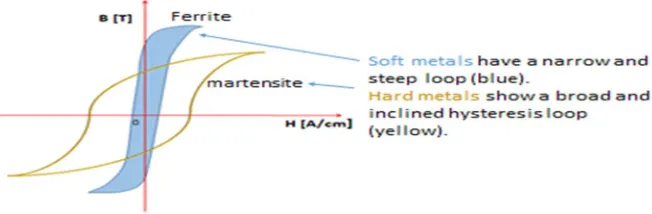
In a hysteresis curve a soft magnetic material having less thin loop because when residual magnetisation is less or small energy loss and therefore a narrow hysteresis loop and magnetisation doesn’t hold for long, while that of a hard magnetic material will be wider because it carry large magnetic field inside it. The reason for the energy loss, characterized by the area inside the hysteresis loop, are residual stress states and all kinds of lattice defects. Lattice defects can occur in the form of dislocation or impurity element with in the metal, including non-ferromagnetic material, which cause an increase in energy loss during the magnetization process. The domain wall are pinned by one-, two- and three- dimension lattice defects and strain stress, caused by macroscopic stress state kind. The Irreversible Block wall movements and turning process contribute to the energy loss and influence of coercivity and remanence values . The dislocation and movability of small scale of angle is compared with Block wall movements , in order to facilitate the understanding of interaction of domain walls with lattice defects and shifting in domain wall movement or jumping process.

Fig. 1.19: The change of the magnetic state (B) of a multi grained, isotropic and ferromagnetic material as function of an applied magnetic field (H), is shown in the hysteresis. Compressive stress causes a widening and inclination of the loop

(yellow). Tensile stress causes a narrowing and increasing slope (blue) [14]

III. EXPERIMENTAL SETUP A. Description

2) Components and Setup: The test setup consists of following micromagnetic measuring system and data acquisition software as shown in Fig.

Fig. (1) MikroMach Sensor/System, (2) supporter/sensor handling, (3) Specimen, (4) USB (A) plug (to PC USB socket, (5) Power supply connector and USB (B) plug; combination plug optional, (6) Data and power supply cable (1.5m length); separate data and

power supply cable optional, (7) Data Acquisition and Analysis software.

3) Measuring System: The inspection technique and standard system components were described in Section above. Fig. Below depicts the individual components of a standard MikroMach system.

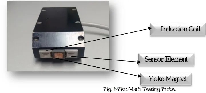
Fig. MikroMach Testing Probe.

a) The yoke (magnet) is used to generate the hysteresis in the material. An alternating magnetic field with adjustable amplitude is created and transferred into the material via the spherical poles.

b) The magnetic field sensor meausres the generated magnetic field strength.

c) The inductive proximity sensor measures the value of the magnetic Barkhausen Noise.

d) The control unit generates the magnetization signal, amplifies and digitizes the measurement signals and transfers the acquired data to the control PC using the USB interface.

e) The MMS software, allows to separate the recorded signals into the 4 different measurement techniques

4) Mechanical Components: The test system can tolerate variable test sample curvatures within certain tolerances, if the sensor element is spring-loaded (optional). Acceptable ranges for curvature radii are specified in the sensor-specific documentation [16]. System applications within this range warrant that both, the yoke magnet and the front of the sensor element are in direct contact with the sample surface, and ensure that slight tilting of the sensor does not impose significant implications. With the exception of the spring-loaded sensor element (optional), the test system does not contain any movable parts.

5) Sensor Components: The sensor and test system are designed in a single unit by Fraunhofer IZFP, suitable for test applications that do not require a separation of sensor and test electronics; various custom-designed configurations are available upon request (Fraunhofer IZFP). Accurate matching of the sensor geometry to the surface geometry of the part(s) to be inspected usually provides an improvement of the calibration accuracy and leads to the concentration of the measurement to the relevant area. The design of the MikroMach model system exhibits a yoke pole size 10mm x 10mm (length, width), and a sensor surface

Sensor Element

Yoke Magnet

area of approximately 10mm x 10mm (length, width). The design of yoke poles and the spring-loaded sensor element permits the testing of curved surfaces.

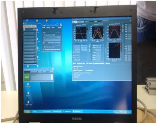
6) Data Acquisition and Analysis Software: the MikroMach system uses the Modular Measurement System (MMS) software, developed by Fraunhofer IZFP. The software separates the measuring process into various modules, e.g. test cycle control, data processing modules and tools, each with its own task. The test cycle control initiates the individual data collection processes in the basic mode, just acting as a start/stop button. The data processing modules provides for the actual data acquisition and data processing functions of the system, i.e. one module for data acquisition, one for data processing and one module for data presentation (results). The tool modules provide for cycle-independent data processing, for example for the presentation of the test results, and are not part of the actual measurement process. The following modules are required to perform basic measurements with the MikroMach system:

Fig. Data Acquisition and Analysis Software displayed on pc screen.

7) Master control unit: The Master control unit manages the system in a cyclic process. The modules like cycle controller, data acquisition and data processing modules are arranged in a loop as shown in the Fig. 2.4 in a cyclic way. When measurements are started the modules are activated one after other as assigned in the master control unit. Each module can process the data of the previous modules. A typical Master control unit is shown in Fig.

Fig. Master control unit

IV. EXPERIMENTAL RESULTS

A. Material list and geometrical description

The different structural I beams with several geometrical specifications and with different mechanical properties are shown below in Table. 1.

Table. 1: Different I beams from structural steels.

B. Measurement and position of testing system

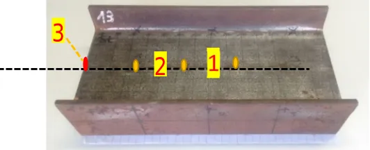
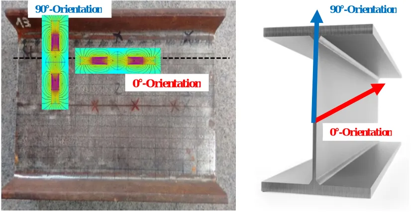
1) Selection of face and position : In our task, the reading analysis is done on web of the symmetrical I-beam steels as shown in Fig. 3.1 as we know, the web resists shear forces, while the flanges resist most of the bending moment experienced by the beam so, the web face is also one of the important scale and and neutral fibre is the middle layer, which do not experience either tension or compression and defines stiffness property so, we have choosen it for our further investigation. On the neutral fibre the points are measured which are at equidistant to each other and the readings are taken at the single points as shown in Fig.

Fig. 3.1 (1) Web, (2) Neutral fibre, (3) measuring point.

2) Use of MikroMach system: Before analysing the characterization of different electromagnetic parameters the measuring and positioning of the MickroMach system has to be carried out and a detailed knowledge regarding the placement has to be adapted depending on the shape of the sample and also type of contact surface of the sample. The placement must be in such a

1

2

way that the contact between the sample surface and the pole shoes of the probe should be without any lift off as shown in the Fig. The issue is to neglect the signal quality at every time of the measurement.

Fig. (a) Contact between the specimen and poles of probe (b) Placement of probe using supporter.

The alignment of probe are of two types which is 0° orientation and 90° orientation because as discussed above in section (1.2.1.3) grain size varies with respect to the rolling direction in the production process.

In a single crystal, the physical and mechanical properties often differ with orientation. It can be seen in the discussion done in section 1.3 of crystalline structure that atoms should be able to slip over one another or distort in relation to one another easier in some directions than others. When the properties of a material vary with different crystallographic orientations, the material is said to be anisotropy.

Fig. 3.3 Illustrate the alignment of probe on the surface of specimen.

3) Selection Of An Optimal Parameter Setup : The parameters like magnetisation frequency, f (Hz) and magnetisation amplitude, H (A/cm) were selected in order to provide a good separation between different I beams. Data collection was performed by using R_Mmax parameters. Barkhausen noise effect, exhibiting a field strength-related gradient, which can be correlated to material yield strength and hardness.In this thesis we examined the different I beams and as it is mentioned in section 2.3 Barkhausen noise signal had a range of 2 to 24 (kHz) with an analysing depth of 10 μm to 1 mm but initially Barkhausen Noise

(BN) signal analysis were done with three different high pass frequency i.e at 2 (kHz), 10 (kHz), 16 (kHz) respectively.Magnetisation amplitude and frequency as well as suitable high pass frequency were investigated and are shown within the following results Fig. 3.4, Fig. 3.5.

(b)

90°-Orientation

0°-Orientation

90°-Orientation

0°-Orientation

Fig. 3.4 (a) At 0° orientation magnetisation amplitude (A/cm) vs R_Mmax (mV) at 2.0 (kHz) high pass frequency, (b) magnetisation amplitude (A/cm) vs R_Mmax (mV) at 10.0 (kHz) high pass frequency.

Fig. 3.5 (c) At 0° orientation magnetisation amplitude (A/cm) vs R_Mmax (mV) At 16.0 (kHz) high pass frequency.

If we compare R_Mmax_1 at 2.0 (kHz), R_Mmax_2 (10 kHz) and R_Mmax_3 (16 kHz) from the result, we can easily observe there is much difference in R_Mmax_3 as compared to R_Mmax_1 , R_Mmax_2 because of high pass frequency and due to very low output dependence to magnetisation amplitude and much scattering in R_Mmax_3 values as shown in Fig. 3.5. So, we neglected the R_Mmax_3.

Then further if we compare the R_Mmax_1 and R_Mmax_2 values as shown in Fig. 3.4 & Fig. 3.5 the output dependence to magnetisation amplitude is somewhat similar but we can observe the scattering is high in R_Mmax_2 compare to R_Mmax_1. So, we can conclude that R_Mmax_1 is the best.

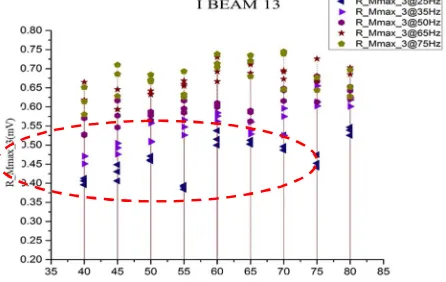
From graph (R_Mmax_1) at 0° orientation. So, we can say that 65 (Hz) and 75 (Hz) frequencies and magnetisation amplitude of 65 (A/cm) and 75 (A/cm) is the best from the results for further investigation of the optimal frequencies and magnetisation amplitude on I beam 13 (Table. 1) in 90° orientation as shown in Fig. 3.6.

Fig.3.6 At 90° orientation magnetisation amplitude (A/cm) vs R_Mmax (mV) at 2.0 kHz high pass frequency.

As per previous results from I beam 13 we came to know about the suitable frequencies (50 Hz to 75 Hz) and optimal magnetisation amplitude i.e. (60 A/cm to 75 A/cm) is the best. For further reading analysis on different I beams we took measurement on particular frequencies and amplitude as mentioned above. Reading analysis is done on I beam 45 at 0° and 90° orientation.

Fig. 3.7 (a) At 0° orientation magnetisation amplitude (A/cm) vs R_Mmax (mV) at 2.0 (kHz) high pass frequency, (b) At 90° orientation magnetisation amplitude (A/cm) vs R_Mmax (mV) at 2.0 (kHz) high pass frequency.

As per the above results at 0°orientationin the marked region of Fig. 3.7 (a) we can see much stable uniform points and they are close enough. Thus it shows optimal frequencies are (65 Hz and 75 Hz) whereas 50 (Hz) is having a low output and optimal magnetization amplitude i.e. (60 A/cm to 75 A/cm) and if we observe in Fig. 3.7 (b) the optimal magnetisation amplitude ranges from (60 A/cm to 65 A/cm) at frequency 65 (Hz).Reading analysis is done on I beam 46 at 0° and 90° orientation.

Fig. 3.8 (a) Magnetisation amplitude (A/cm) vs R_Mmax (mV) at 2.0 (kHz) high pass frequency a 0° orientation, (b) magnetisation amplitude (A/cm) vs R_Mmax (mV) at 2.0 (kHz) high pass frequency at 90° orientation.

As shown in Fig. 3.8 the results at 0° orientation in the marked region (a) we can see stable uniform points and they are close enough, thus it shows optimal frequency is (65 Hz) and optimal magnetisation amplitude i.e., (75 A/cm) and (b) the optimal magnetisation amplitude is (75 A/cm) and frequency is 65 Hz.Further investigation is done on I beam 56. To know the influence on electromagnetic parameters the measurements are taken on the I beam 56 at different elevation of temperature i.e. 20°C, 50°C and 75°C. A heat blower is used to heat the surface of specimen to 50°C and 75°C. To measure the temperature of beam thermocouple is

used. The process of heating the steel beam using a heat blower is illustrated in the below Fig. 3.9.

(a)

(b)

,

(a) (b)

Fig. 3.9 (a) (1) Blower (2) Thermocouple, (b) Display of temperature reading.

The influence of parameters can be observed at different temperatures as shown in Fig. 3.10.

Fig. 3.10 (a) Magnetisation amplitude (A/cm) vs R_Mmax_1 (mV) at 50 (Hz)

(b) Magnetisation amplitude (A/cm) vs R_Mmax_1 (mV) at 65 (Hz).

Fig. 3.11. Magnetisation amplitude (A/cm) vs R_Mmax_1 (mV) at 75(Hz).

As shown in Fig. 3.10 (a) R_Mmax_1 values with varying temperature at 0° orientation 20°C values are highly scattered compared to 50°C and 75°C. The high R_Mmax_1 values are noted in 20°C of 50 (Hz) Fig. 3.10 (b) there is a less scattering in 75°C and 50°C at 0° orientation of 65 (Hz) but output is low in 75°C dependence to magnetisation amplitude. At 75 (A/cm) and 80 (A/cm) the scattering of R_Mmax_1 values are less at 65 (Hz). Fig. 3.11 from 55 (A/cm) to 60 (A/cm) the values are less scattered compared to other magnetisation amplitudes of 75 (Hz).

1

2

(a) (b) Fig. 3.12 (a) Magnetisation amplitude (A/cm) vs R_Mmean_1 (mV) at 50 (Hz)

(b) Magnetisation amplitude (A/cm) vs R_Mmean_1 (mV) at 65 (Hz).

Fig. 3.13. Magnetisation amplitude (A/cm) vs R_Mmean_1 (mV) at 75 (Hz).

(a) (b)

Fig. 3.14 (a) Magnetisation amplitude (A/cm) vs R_Vmag (mV) at 50 (Hz) (b) Magnetisation amplitude (A/cm) vs R_Vmag (mV) at 65 (Hz).

Fig. 3.15 Magnetisation amplitude (A/cm) vs R_Vmag (mV) at 75 (Hz).

Fig. 3.14 (a) R_Vmag values are linear and gradually increases at 50 (Hz) with increases in magnetisation amplitude. (b) In 20°C at 0° orientation the values having a low output from 65 (A/cm) to 70 (A/cm) whereas in Fig. 3.15 the output is low at 40 (A/cm) to 45 (A/cm) for 20°C at 90° orientation.

V. CONCLUSION

A. By this investigation it can be concluded that at less temperature the influence is more in most of the measured parameters. B. Scatter values of measured parameters at 20°C is more as compared to other temperature and output differs as well. C. With these investigation it can be concluded the temperature should be considered while measurement are done.

REFERENCES

[1] Starke, P. (2017). Metallic Materials. Lecture.

[2] “Corrosion.” [Online]. Available: www.chemistryexplained.com/Co-Di/Corrosion.htm

[3] “Properties of Steel.” [Online]. Available: https://en.wikipedia.org/wiki/Structural_steel#cite_note- _of_Structural_Engineerin [4] Magnetism and Magnetic Materials – J. M. D. Coey

[5] R. L. Stamps, “Magnetism,” Springer International Publishing, 2013, pp. 1-49. [6] Atomic Structure – E. U. Condon, Halis Odabasi

[7] Kankanti, Kiran Prateek.” Non-Destructive of steel piping components by Metal Magnetic Memory (MMM) Technique. Master's thesis, RWTH Aachen University of Technology Institute of Ironworks, 2010

[8] A. Hubert and R. Schafer, Magnetic Domains: The Analysis Magnetic Microstructures – Alex Hubert, Rudolf Schafe [9] L. Li,”Stress effect on ferromagnetic materials: investigation of stainless steel and nickel,” Retrosp. Thesis Diss., 200