On Model Stability as a Function of Random Seed

929

On Model Stability as a Function of Random Seed

Pranava Madhyastha Department of Computing

Imperial College London

[email protected]

Rishabh Jain∗ Bloomberg

London

[email protected]

Abstract

In this paper, we focus on quantifying model stability as a function of random seed by in-vestigating the effects of the induced random-ness on model performance and the robustrandom-ness of the model in general. We specifically per-form a controlled study on the effect of random seeds on the behaviour of attention, gradient-based and surrogate model gradient-based (LIME) in-terpretations. Our analysis suggests that ran-dom seeds can adversely affect the consistency of models resulting in counterfactual interpre-tations. We propose a technique called Aggres-sive Stochastic Weight Averaging (ASWA)and an extension calledNorm-filtered Aggressive Stochastic Weight Averaging (NASWA)which improves the stability of models over random seeds. With our ASWA and NASWA based optimization, we are able to improve the ro-bustness of the original model, on average re-ducing the standard deviation of the model’s performance by72%.

1 Introduction

There has been a tremendous growth in deep neu-ral network based models that achieve state-of-the-art performance. In fact, most recent end-to-end deep learning models have surpassed the performance of careful human feature-engineering based models in a variety of NLP tasks. However, deep neural network based models are often brit-tle to various sources of randomness in the training of the models. This could be attributed to several sources including, but not limited to, random pa-rameter initialization, random sampling of exam-ples during training and random dropping of neu-rons. It has been observed that these models have, more often, a set ofrandom seedsthat yield better results than others. This has also lead to research

∗

This work was conducted when the author was a student at Imperial College London.

suggesting random seeds as an additional hyper-parameter for tuning (Bengio,2012)1_{. One} possi-ble explanation for this behavior could be the exis-tence of multiple local minima in the loss surface. This is especially problematic as the loss surfaces are generally non-convex and may have multiple saddle points making it difficult to achieve model stability.

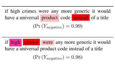
if high crimes were any more generic it would have a universal product code instead of a title

(Pr (Ynegative) = 0.99)

if high crimes were any more generic it would have a universal product code instead of a title

(Pr (Ynegative) = 0.98)

Figure 1: Importance based on attention

probabil-ities for two runs of the same model with same

parameters and same hyperparameters, but with

two different random seeds (color magnitudes: pink<magenta<red)

Recently the NLP community has witnessed a resurgence in interpreting and explaining deep neural network based models (Jain et al., 2019;

Jain and Wallace, 2019; Alvarez-Melis and Jaakkola,2017). Most of the interpretation based methods involve one of the following ways of in-terpreting models: a) sample oriented interpreta-tions: where the interpretation is based on changes in the prediction score with either upweighting or perturbing samples (Jain et al., 2019;Jain and Wallace,2019;Koh and Liang,2017); b) interpre-tations based on feature attributions using atten-tion or input perturbaatten-tion or gradient-based mea-sures; (Ghaeini et al., 2018; Feng et al., 2018;

Bach et al.,2015); c) interpretations using

surro-1_{http://www.argmin.net/2018/02/26/}

gate linear models (Ribeiro et al., 2016) – these methods can provide local interpretations based on input samples or features. However, the presence of inherent randomness makes it difficult to accu-rately interpret deep neural models among other forms of pathologies (Feng et al.,2018).

In this paper, we focus on the stability of deep neural models as a function of random-seed based effects. We are especially interested in investigat-ing the hypothesis focusinvestigat-ing on model stability: do neural network based models under different ran-dom seeds allow for similar interpretations of their decisions? We claim that for a given model which achieves a substantial performance for a task, the factors responsible for any decisions over a sam-ple should be approximately consistent irrespec-tive of the random seed. In Figure 1, we show an illustration of this question where we visual-ize the attention distributions of two CNN based binary classification models for sentiment anal-ysis, trained with the same settings and hyper-parameters, but withdifferent seeds. We observe that both models obtain the correct prediction with significantly high confidence. However, we note that both the models attend to completely differ-ent sets of words. This is problematic, especially when interpreting these models under the influ-ence of such randomness. We observe that on av-erage40−60%of the most important interpretable units are different across different random seeds for the same model. This phenomenon also leads us to the question on the exact nature of inter-pretability – are the interpretations specific to an instantiation of the model or are they general to a class of models?

We also provide a simple method that can, to a large extent, ameliorate this inherent random behaviour. In Section 3.1, we propose an ag-gressive stochastic weight averaging approach that helps in improving the stability of the models at almost zero performance loss while still making the model robust to random-seed based instability. We also propose an improvement to this model in Section3.2which further improves the stability of the neural models. Our proposals significantly im-prove the robustness of the model, on average by

72%relative to the original model and on Diabetes (MIMIC), a binary classification dataset, by89%

(relative improvement). All code for reproducing and replicating our experiments is released in our

repository2.

2 Measuring Model Stability

In this section, we describe methods that we use to measure model stability, specifically — prediction and interpretation stability.

2.1 Prediction Stability

We measure prediction stability using standard measures of the mean and the standard deviations corresponding to the accuracy of the classification based models on different datasets. We ensure that the models are run with exactly the same config-urations and hyper-parameters but with different random seeds. This is a standard procedure that is used in the community to report the performance of the model.

2.2 Interpretation Stability

For a given task, we train a set of models only differing with random-seeds. For every given test sample, we obtain interpretations using different instantiations of the models. We define a model to be stable if we obtain similar interpretations re-gardless of different random-seed based instanti-ations. We use the following metrics to quantify stability:

a) Relative Entropy quantification (H): Given two distributions over interpretations, for the same test case, from two different models, it measures the relative entropy between the two probability distributions. Note that, the higher the relative entropy the greater the dissimilarity be-tween the two distributions.

H=X

i∈d

Pr1·log

Pr1

Pr2

where,Pr1andPr2are two attention distributions

of the same sample from two different runs of the model anddis the number of tokens in the sam-ple. Givenndifferently seeded models, for each test instance, we calculate the relative entropy ob-tained from the corresponding averaged pairwise interpretation distributions.

b)Jaccard Distance (J): It measures the dis-similarity between two sets. Here higher values ofJ indicate larger variances. We consider top-n

tokens which have the highest attention for com-parison. Note that, Jaccard distance is over sets of

word indices and do not take into account the at-tention probabilities explicitly. Jaccard distance is defined as:

J = (1−A∩B

A∪B)∗100%

where, A and B are the sets of most relevant items. We specifically decided to use ‘most’ rel-evant (top-n items) as the tail of the distribution mostly consists of values close to0.

Interpretation methods under study: In this paper we study interpretation stability using the following three interpretation methods:

1. Attention based interpretation: We focus on attention probabilities as the mode of inter-pretation and consider the model to be stable if different instantiations of the model leads to similar attention distributions. Our major focus in this paper is attention based inter-pretation. As we use Jain et al. (2019) as a testbed for our investigation, we focus heav-ily on attention. Also, as the attention layer has a linear relationship with the prediction, we consider attention to be more indicative of the model stability.

2. Gradient-based feature importance: Given a sample, we use the input gradients of the model corresponding to each of the word rep-resentations and compute the magnitude of the change as a local explanation. We re-fer the reader to Baehrens et al. (2010) for a good introduction to gradient-based inter-pretations. As all of our models are differen-tiable, we use this as an alternative method for interpretation. We follow the standard procedure as followed in Feng et al. (2018) and note that we do not followJain and Wal-lace (2019) and do not disconnect the com-putational graph at the attention module. We obtain probabilistic gradient scores by nor-malizing over the absolute values of gradient values.

3. LIME based interpretation: We use lo-cally interpretable model-agnostic interpreta-tions (Ribeiro et al.,2016) that learns a sur-rogate interpretable model locally around the predictions of the deep neural based model. We obtain LIME based interpretations for ev-ery instantiation of the models. We then use Jaccard Distance to measure the divergence.

We note that, we observe similar patterns across the three interpretation methods and the interpre-tations consistently differ with random seeds.

3 Reducing Model Instability with an Optimization Lens

We observe that different instantiations of the model can cause the model have different starts on the optimization surface. Further, stochastic sampling might result in different paths. Both of these factors can lead to different local minimas potentially leading to different solutions. With this observation as our background we propose two, closely related, methods to ameliorate di-vergence: Agressive Stochastic Weight Averaging and Norm-filtered Agressive Stochastic Weight Averaging. We describe these two in the follow-ing subsections.

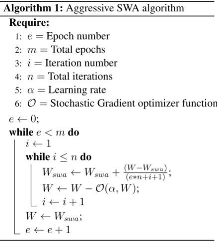
3.1 Aggressive Stochastic Weight Averaging (ASWA)

Stochastic weight averaging (SWA) (Izmailov et al., 2018) works by averaging the weights of multiple points in the trajectory of gradient de-scent based optimizers. The algorithm typically uses modified learning rate schedules. SWA is itself based on the idea of maintaining a run-ning average of weights in stochastic gradient descent based optimization techniques (Ruppert,

1988;Polyak and Juditsky, 1992). The principle idea in SWA is averaging the weights that are max-imally distant helps stabilize the gradient descent based optimizer trajectory and improves general-ization. Izmailov et al. (2018) use the analysis ofMandt et al.(2017) to illustrate the stability ar-guments where they show that, under certain con-vexity assumptions, SGD iterations can be visual-ized as sampling from a Gaussian distribution cen-tred at the minimaof the loss function. Samples from high-dimensional Gaussians are expected to be concentratedon the surface of the ellipse and not close to the mean. Averaging iterations is shown to stabilize the trajectory and further im-prove the width of the solutions to be closer to the

mean.

the conditions for the optimizer and assume that the optimizer is based on some version of gradi-ent descgradi-ent — this means that our modification is valid even for other pseudo-first-order optimiza-tion algorithms including Adam (Kingma and Ba,

2014) and Adagrad (Duchi et al.,2011).

We note that, Izmailov et al. (2018) suggest using SWA usually after ’pre-’training the model (at least until75% convergence) and followed by sampling weights at different steps either using large constant or cyclical learning rates. While, SWA is well defined for convex losses (Polyak and Juditsky, 1992), Izmailov et al. (2018) con-nect SWA to non-convex losses by suggesting that the loss surface isapproximatelyconvex after con-vergence. In our setup, we investigate the utility of averaging weights over every iteration (an it-eration consists of one batch of the gradient de-scent). Algorithm 1 shows the implementation pseudo-code for SWA. We note that, unlike Iz-mailov et al. (2018), we average our weights at

each batchupdate and assign the ASWA parame-ters to the model at the end of each epoch. That is, we replace the model’s weights for the next epoch with the averaged weights.

Algorithm 1:Aggressive SWA algorithm Require:

1: e=Epoch number

2: m=Total epochs 3: i=Iteration number 4: n=Total iterations

5: α=Learning rate

6: O=Stochastic Gradient optimizer function

e←0;

whilee < mdo

i←1

whilei≤ndo

Wswa←Wswa+(W_(e∗−_n+i+1)Wswa);

W ←W − O(α, W);

i←i+ 1 W ←Wswa;

e←e+ 1

In Figure 2, we show an SGD optimizer (with momentum) and the same optimizer with SWA

over a 3-dimensional loss surface with a saddle point. We observe that the original SGD reaches the desired minima, however, it almost reaches the saddle point and does a course correction and reaches minima. On the other hand, we observe

that SGD with ASWA is very conservative, it re-peatedly restarts and reaches the minima without reaching the saddle point. We empirically ob-serve that this is a desired property for the sta-bility of models over runs of the same model that differ only over random instantiations. The grey circles in Figure2highlight this conservative behaviour of SGD with ASWA optimizer, espe-cially when compared to the standard SGD. Fur-ther, Polyak and Juditsky (1992) show that for convex losses, averaging SGD proposals achieves the highest possible rate of convergence for a vari-ety of first-order SGD based algorithms.

(a) Trajectory for Stochastic Gradient Descent

(b) Trajectory for Stochastic Gradient Descent with ASWA

Figure 2: Trajectory for gradient descent algorithms with red and black arrows on (b) indicating movements from consecutive epochs with restarts. Conservative behaviour of ASWA algorithm helps avoid the saddle point without ever reaching it.

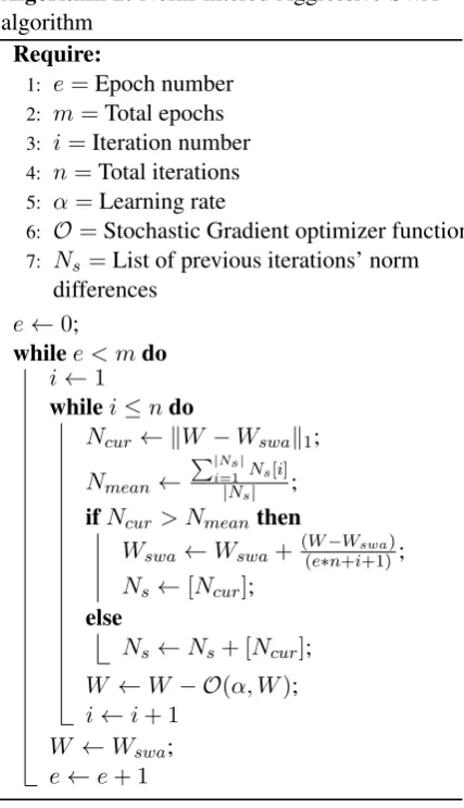
3.2 Norm-filtered Aggressive Stochastic Weight Averaging (NASWA)

Algorithm 2:Norm-filtered Aggressive SWA algorithm

Require:

1: e=Epoch number 2: m=Total epochs 3: i=Iteration number

4: n=Total iterations 5: α=Learning rate

6: O=Stochastic Gradient optimizer function

7: Ns=List of previous iterations’ norm

differences

e←0;

whilee < mdo

i←1

whilei≤ndo

Ncur← kW −Wswak1;

Nmean←

P|Ns|

i=1 Ns[i]

|Ns| ;

ifNcur> Nmeanthen

Wswa ←Wswa+ (W_(e∗−_n+i+1)Wswa);

Ns←[Ncur]; else

Ns←Ns+ [Ncur];

W ←W − O(α, W);

i←i+ 1 W ←Wswa;

e←e+ 1

maintain a list that stores the norm differences of the previous iterations. If the norm difference of the current iteration is greater than the average of the list, we update the ASWA weights and reini-tialize the list with the current norm difference. When the norm difference, however, is less than the average of the list, we just append the current norm difference to the list. After the completion of the epoch, we assign the ASWA parameters to the model. This is shown in Algorithm2. We call this approachNorm-filtered Aggressive Stochastic Weight Averaging.

4 Experiments

We base our investigation on similar sets of mod-els asJain and Wallace (2019). We also use the code provided by the authors for our empirical in-vestigations for consistency and empirical valida-tion. We describe our models and datasets used for the experiments below.

4.1 Models

We consider two sets of commonly used neural models for the tasks of binary classification and multi-class natural language inference. We use CNN and bi-directional LSTM based models with attention. We follow (Jain and Wallace,2019) and use similar attention mechanisms using a) additive attention (Bahdanau et al.,2014); and b) scaled dot product based attention (Vaswani et al.,2017). We jointly optimize all the parameters for the model, unlikeJain and Wallace(2019) where the encod-ing layer, attention layer and the output prediction layer are all optimized separately. We experiment with several optimizers including Adam (Kingma and Ba, 2014), SGD and Adagrad (Duchi et al.,

2011) but most results below are with Adam. For our ASWA and NASWA based experi-ments, we use a constant learning rate for our op-timizer. Other model-specific settings are kept the same asJain and Wallace(2019) for consistency.

Dataset Avg. Length Train Size Test size

IMDB 179 12500 / 12500 2184 / 2172

Diabetes(MIMIC) 1858 6381 / 1353 1295 / 319

SST 19 3034 / 3321 652/653

Anemia(MIMIC) 2188 1847 / 3251 460 / 802

AgNews 36 30000 / 30000 1900 / 1900

ADR Tweets 20 14446 / 1939 3636 / 487

SNLI 14 182764 / 183187 / 183416 3219 / 3237 / 3368

Table 1: Dataset characteristics. Train size and test size show the cardinality for each class. SNLI is a three-class dataset while the rest are binary three-classification

4.2 Datasets

The datasets used in our experiments are listed in Table 1 with summary statistics. We fur-ther pre-process and tokenize the datasets us-ing the standard procedure and follow Jain and Wallace (2019). We note that IMDB (Maas et al., 2011), Diabetes(MIMIC) (Johnson et al.,

2016), Anemia(MIMIC) (Johnson et al., 2016), AgNews (Zhang et al.,2015), ADR Tweets ( Nik-farjam et al.,2015) and SST (Socher et al.,2013) are datasets for the binary classification setup. SNLI (Bowman et al., 2015) is a dataset for the multiclass classification setup. All of the datasets are in English, however we expect the behavior to persist regardless of the language.

4.3 Settings and Hyperparameters

We use a 300-dimenstional embedding layer which is initialized with FastText (Joulin et al.,

We use a128-dimensional hidden layer for the bi-directional LSTM and a32-dimensional filter with kernels of size{1,3,5,7}for CNN. For others, we maintain the model settings to resemble the mod-els inJain and Wallace(2019). We train all of our models for 20 Epochs with a constant batch size of 32. We use early stopping based on the valida-tion set using task-specific metrics (Binary Classi-fication: usingroc-auc, Multiclass and question answering based dataset: usingaccuracy).

Dataset CNN(%) CNN+ASWA(%) CNN+NASWA(%)

IMDB 89.8 (±0.79) 90.2 (±0.25) 90.1 (±0.29) Diabetes 87.4 (±2.26) 85.9 (±0.25) 85.9 (±0.38) SST 82.0 (±1.01) 82.5 (±0.39) 82.5 (±0.39) Anemia 90.6 (±0.98) 91.9 (±0.20) 91.9 (±0.19) AgNews 95.5 (±0.23) 96.0 (±0.11) 96.0 (±0.07) Tweet 84.6 (±2.65) 84.4 (±0.54) 84.4 (±0.54)

Table 2: Performance statistics obtained from 10 dif-ferently seeded CNN based models. Table compares accuracy and itsstandard deviationfor the normally trained CNN model against the ASWA and NASWA trained models, whose deviation drops significantly, thus, indicating increased robustness.

5 Results

In this section, we summarize our findings for10

runs of the model with10 different random seeds but with identical model settings.

5.1 Model Performance and Stability

We first report model performance and prediction stability. The results are reported in Table2.

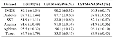
Dataset LSTM(%) LSTM+ASWA(%) LSTM+NASWA(%)

IMDB 89.1 (±1.34) 90.2 (±0.32) 90.3 (±0.17) Diabetes 87.7 (±1.44) 87.7 (±0.60) 87.8 (±0.55) SST 81.9 (±1.11) 82.0 (±0.60) 82.1 (±0.57) Anemia 91.6 (±0.49) 91.8 (±0.34) 91.9 (±0.36) AgNews 95.5 (±0.32) 96.1(±0.17) 96.1 (±0.10) Tweet 84.7 (±1.79) 83.8 (±0.45) 83.9 (±0.45)

Table 3: Performance statistics obtained from 10 dif-ferently seeded LSTM based models.

We note that the original CNN based mod-els, on an average, have a standard deviation of ±1.5%. Which seems standard, however, we note that ADR Tweets dataset has a very high standard deviation of±2.65%. We observe that ASWA and NASWA are almost always able to achieve higher performance with a very low standard deviation. This suggests that both ASWA and NASWA are extremely stable when compared to the standard model. They significantly improve the robustness, on an average, by 72% relative to the original

model and on Diabetes (MIMIC), a binary clas-sification dataset, by89%(relative improvement). We observe similar results for the LSTM based models in Table3.

(a) CNN models (b) LSTM models

Figure 3: Prediction’s standard deviation for CNN and LSTM based models for all binary classification datasets under consideration. Predictions are bucketed in intervals of size 0.1, starting from 0 (containing pre-dictions from 0 to 0.1), until 0.9

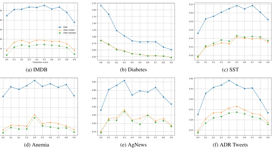
We further analyze the prediction score stabil-ity by computing the mean standard deviation over the binned confidence intervals of the models in Figure3a. We note that on an average, the stan-dard deviations are on the lower side. However, we observe that the mean standard deviation of the bins close to0.5is on the higher side as is expected given the high uncertainty. On the other hand both, ASWA and NASWA based models are rel-atively more stable than the standard CNN based model. We observe similar behaviours for the LSTM based models in Figure3b. This suggests that our proposed methods, ASWA and NASWA, are able to obtain relatively better stability without any loss in performance. We also note that both ASWA and NASWA had relatively similar perfor-mance over more than10random seeds.

5.2 Attention Stability

(a) CNN models (b) LSTM models

We now consider the stability of attention dis-tributions as a function of random seeds. We first plot the results of the experiments for standard

CNN based binary classification models over uni-formly binned prediction scores for positive labels in Figure4a. We observe that, depending on the datasets, the attention distributions can become extremely unstable (high entropy). We specifi-cally highlight the Diabetes(MIMIC) dataset’s en-tropy distribution. We observe similar, but rela-tively worse results for the LSTM based models in Figure4b. In general, we would expect the en-tropy distribution to be close to zero however, this doesn’t seem to be the case. This means that using attention distributions to interpret models may not be reliable and can lead to misinterpretations.

(a) CNN models (b) LSTM models

Figure 5: Jaccard distance highlighting instability in at-tention distributions of CNN and LSTM based models.

(a) CNN+ASWA (b) CNN+NASWA

(c) LSTM+ASWA (d) LSTM+NASWA

Figure 6: Improved prediction stability from ASWA and NASWA for CNN and LSTM based models

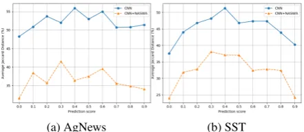
We use the top 20% of the most important items (indices) in the attention distribution for each dataset over10runs and plot the Jaccard dis-tances for CNN and LSTM based models in Fig-ure 5a and Figure5b. We again notice a similar

(a) Diabetes (b) SST

Figure 7: Gradient based interpretations’ stability im-provement from NASWA on CNN based models. The Jaccard distance is calculated using the top 20% atten-tive items.

trend of unstable attention distributions over both CNN and LSTM based attention distribution.

In the following sections for space constraints, we focus on CNN based models with additive at-tention. Our results on LSTM based models are provided in the attached supplementary material. We note that the observations for LSTM mod-els are, in most cases, similar to the behaviour of the CNN based models. Scaled dot-product based models are also provided in the supplemen-tary material and we notice a similar trend as the additive attention.

We now focus on the effect of ASWA and NASWA on binary and multi-class CNN based neural models separately.

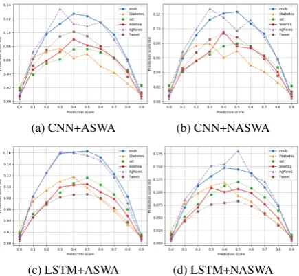
Binary Classification In Figure 8, we plot the results of the models with ASWA and NASWA. We observe that both these algorithms signifi-cantly improve the model stability and decrease the entropy between attention distributions. For example, in Figure8b, both ASWA and NASWA decrease the average entropy by about60%. We further notice that NASWA is slightly better per-forming in most of the runs. This empirically val-idates the hypothesis that averaging the weights from divergent weights (when the norm difference is higher than the average norm difference) helps in stabilizing the model’s parameters, resulting in a more robust model.

(a) IMDB (b) Diabetes (c) SST

(d) Anemia (e) AgNews (f) ADR Tweets

Figure 8: Attention stability improvement from ASWA and NASWA on CNN based models.

(a) Label 0 prediction vs entropy (b) Label 1 prediction vs entropy (c) Label 2 prediction vs entropy

Figure 9: Attention stability improvement from ASWA and NASWA on CNN based model for the SNLI dataset.

with random seeds.

5.3 Gradient-based Interpretations

We now look at an alternative method of interpret-ing deep neural models and look into the consis-tency of the gradient-based interpretations to fur-ther analyze the model’s instability. For this setup, we focus on binary classifier and plot the results on the SST and the Diabetes dataset in partic-ular since they cover the low and the high end of the entropy spectrum (respectively). We no-tice similar trends of instability in the gradient-based interpretations from model inputs as we did for the attention distributions. Figure 7 shows that the entropy between the gradient-based inter-pretations from differently seeded models closely follows the same trend as the attention distribu-tions. This result further strengthens our claim on the importance of model stability and shows that over different runs of the same model with

differ-ent seeds, we may get differdiffer-ent interpretations us-ing gradient-based feature importance. Moreover, Figure7shows the impact of ASWA towards mak-ing the gradient-based interpretations more consis-tent, thus, significantly increasing the stability.

5.4 LIME based Interpretations

(a) AgNews (b) SST

Figure 10: LIME based interpretations’ stability im-provement from NASWA on CNN based models. The Jaccard distance is calculated using the top 20% atten-tive items.

observe once again that NASWA helps in reduc-ing the instability and results in more consistent interpretations.

In all our experiments, we find that a significant proportion of interpretations are dependent on the instantiation of the model. We also note that we perform experiments over 100random seeds for greater statistical power and see similar patterns3_.

6 Discussion

Recent advances in adversarial machine learn-ing (Neelakantan et al.,2015;Zahavy et al.,2016) have investigated robustness to random initializa-tion based perturbainitializa-tions, however, to our knowl-edge, no previous study investigates the effect of random-seeds and its connection on model inter-pretation. Our study analyzed the inherent lack of robustness in deep neural models for NLP. Recent studies cast doubt on the consistency and corre-lations of several types of interpretations ( Doshi-Velez and Kim, 2017; Jain and Wallace, 2019;

Feng et al.,2018). We hypothesise that some of these issues are due to the inherent instability of the deep neural models to random-seed base per-turbations. Our analysis (in Section 4) leads to the hypothesis that models with different instanti-ations may use completely different optimization paths. The issue of variance in all black-box in-terpretation methods over different seeds will con-tinue to persist until the models are fully robust to random-seed based perturbations. Our work how-ever, doesn’t provide insights into instabilities of different layers of the models. We hypothesise that it might further uncover the reasons for the rela-tively lower correlation between different black-box interpretation methods as these are effectively based off on different layers and granularity.

3_{These results are provided in the appendix.}

There has been some work on using noisy gradi-ents (Neelakantan et al.,2015) and learning from adversarial and counter-factual examples (Feng et al., 2018) to increase the robustness of deep learning models.Feng et al.(2018) show that neu-ral models may use redundant features for predic-tion and also show that most of the black-box in-terpretation methods may not be able to capture these second-order effects. Our proposals show that aggressively averaging weights leads to bet-ter optimization and the resultant models are more robust to random-seed based perturbation. How-ever, our research is limited to increasing consis-tency in neural models. Our approach further uses first order based signals to boost stability. We posit that second-order based signals can further enhance consistency and increase the robustness.

7 Conclusions

In this paper, we study the inherent instability of deep neural models in NLP as a function of ran-dom seed. We analyze model performance and robustness of the model in the form of attention based interpretations, gradient-based feature im-portance and LIME based interpretations across multiple runs of the models with different random seeds. Our analysis strongly highlights the prob-lems with stability of models and its effects on black-box interpretation methods leading to differ-ent interpretations for differdiffer-ent random seeds. We also propose a solution that makes use of weight averaging based optimization technique and fur-ther extend it with norm-filtering. We show that our proposed methods largely stabilize the model to random-seed based perturbations and, on aver-age, significantly reduce the standard deviations of the model performance by72%. We further show that our methods significantly reduce the entropy in the attention distribution, the gradient-based feature importance measures and LIME based in-terpretations across runs.

Acknowledgments

References

David Alvarez-Melis and Tommi S Jaakkola. 2017. A causal framework for explaining the predictions

of black-box sequence-to-sequence models. arXiv

preprint arXiv:1707.01943.

Sebastian Bach, Alexander Binder, Grégoire Mon-tavon, Frederick Klauschen, Klaus-Robert Müller, and Wojciech Samek. 2015. On pixel-wise explana-tions for non-linear classifier decisions by layer-wise relevance propagation. PloS one, 10(7):e0130140.

David Baehrens, Timon Schroeter, Stefan Harmel-ing, Motoaki Kawanabe, Katja Hansen, and Klaus-Robert MÞller. 2010. How to explain individual classification decisions. Journal of Machine Learn-ing Research, 11(Jun):1803–1831.

Dzmitry Bahdanau, Kyunghyun Cho, and Yoshua

Ben-gio. 2014. Neural machine translation by jointly

learning to align and translate. arXiv preprint

arXiv:1409.0473.

Yoshua Bengio. 2012. Practical recommendations for gradient-based training of deep architectures. In

Neural networks: Tricks of the trade, pages 437– 478. Springer.

Samuel R Bowman, Gabor Angeli, Christopher Potts, and Christopher D Manning. 2015. A large anno-tated corpus for learning natural language inference.

arXiv preprint arXiv:1508.05326.

Finale Doshi-Velez and Been Kim. 2017. Towards a rigorous science of interpretable machine learning.

arXiv preprint arXiv:1702.08608.

John Duchi, Elad Hazan, and Yoram Singer. 2011. Adaptive subgradient methods for online learning

and stochastic optimization. Journal of Machine

Learning Research, 12(Jul):2121–2159.

Shi Feng, Eric Wallace, Alvin Grissom II, Pedro Rodriguez, Mohit Iyyer, and Jordan Boyd-Graber. 2018. Pathologies of neural models make interpreta-tion difficult. InEmpirical Methods in Natural Lan-guage Processing.

Reza Ghaeini, Xiaoli Z Fern, and Prasad Tadepalli.

2018. Interpreting recurrent and attention-based

neural models: a case study on natural language in-ference.arXiv preprint arXiv:1808.03894.

Pavel Izmailov, Dmitrii Podoprikhin, Timur Garipov, Dmitry Vetrov, and Andrew Gordon Wilson. 2018. Averaging weights leads to wider optima and better generalization. arXiv preprint arXiv:1803.05407.

Sarthak Jain, Ramin Mohammadi, and Byron C

Wal-lace. 2019. An analysis of attention over

clin-ical notes for predictive tasks. arXiv preprint

arXiv:1904.03244.

Sarthak Jain and Byron C. Wallace. 2019. Attention is not explanation.CoRR, abs/1902.10186.

Alistair EW Johnson, Tom J Pollard, Lu Shen,

H Lehman Li-wei, Mengling Feng,

Moham-mad Ghassemi, Benjamin Moody, Peter Szolovits, Leo Anthony Celi, and Roger G Mark. 2016. Mimic-iii, a freely accessible critical care database.

Scientific data, 3:160035.

Armand Joulin, Edouard Grave, Piotr Bojanowski, Matthijs Douze, Hérve Jégou, and Tomas Mikolov. 2016. Fasttext. zip: Compressing text classification models. arXiv preprint arXiv:1612.03651.

Diederik P Kingma and Jimmy Ba. 2014. Adam: A method for stochastic optimization. arXiv preprint arXiv:1412.6980.

Pang Wei Koh and Percy Liang. 2017. Understand-ing black-box predictions via influence functions. InProceedings of the 34th International Conference on Machine Learning-Volume 70, pages 1885–1894. JMLR. org.

Andrew L Maas, Raymond E Daly, Peter T Pham, Dan Huang, Andrew Y Ng, and Christopher Potts. 2011. Learning word vectors for sentiment analysis. In

Proceedings of the 49th annual meeting of the as-sociation for computational linguistics: Human lan-guage technologies-volume 1, pages 142–150. Asso-ciation for Computational Linguistics.

Stephan Mandt, Matthew D Hoffman, and David M Blei. 2017. Stochastic gradient descent as

approx-imate bayesian inference. The Journal of Machine

Learning Research, 18(1):4873–4907.

Arvind Neelakantan, Luke Vilnis, Quoc V Le, Ilya Sutskever, Lukasz Kaiser, Karol Kurach, and James

Martens. 2015. Adding gradient noise improves

learning for very deep networks. arXiv preprint

arXiv:1511.06807.

Azadeh Nikfarjam, Abeed Sarker, Karen O’connor, Rachel Ginn, and Graciela Gonzalez. 2015. Phar-macovigilance from social media: mining adverse drug reaction mentions using sequence labeling

with word embedding cluster features. Journal

of the American Medical Informatics Association, 22(3):671–681.

Boris T Polyak and Anatoli B Juditsky. 1992.

Ac-celeration of stochastic approximation by averag-ing. SIAM Journal on Control and Optimization, 30(4):838–855.

Marco Tulio Ribeiro, Sameer Singh, and

Car-los Guestrin. 2016. Model-agnostic

inter-pretability of machine learning. arXiv preprint

arXiv:1606.05386.

David Ruppert. 1988. Stochastic approximation.

Technical report, Cornell University Operations Re-search and Industrial Engineering.

Richard Socher, Alex Perelygin, Jean Wu, Jason Chuang, Christopher D Manning, Andrew Ng, and

for semantic compositionality over a sentiment

tree-bank. In Proceedings of the 2013 conference on

empirical methods in natural language processing, pages 1631–1642.

Ashish Vaswani, Noam Shazeer, Niki Parmar, Jakob Uszkoreit, Llion Jones, Aidan N Gomez, Łukasz Kaiser, and Illia Polosukhin. 2017. Attention is all

you need. InAdvances in neural information

pro-cessing systems, pages 5998–6008.

Tom Zahavy, Bingyi Kang, Alex Sivak, Jiashi Feng, Huan Xu, and Shie Mannor. 2016. Ensemble robust-ness and generalization of stochastic deep learning algorithms.arXiv preprint arXiv:1602.02389.