ISSN: 1816-949X
© Medwell Journals, 2020
Multi-Floor Facility Layout Problems Solving by the
Differential Evolution Method
1
Jittraporn Palakawong Na Ayutthaya,
1Nuchsara Kriengkorakot,
1Preecha Kriengkorakot and
2Prasert Sriboonchandr
1Department of Industrial Engineering, Faculty of Engineering,
Ubon Ratchathani University, 34190 Ubon Ratchathani, Thailand
2Department of Industrial Engineering, Faculty of Industrial Technology and Management,
King Mongkut’s University of Technology North Bangkok (Prachinburi Campus),
Bangkok, Thailand
Abstract: This research aimed to study the Differential Evolution (DE) for solving the Multi-floor Facility Layout Problem. (MFLP) with the target of minimize the transporting material cost.The DE algorithm had been evaluated and would be compared with MULTIPLE and SABLE algorithm. For MFLP, the Differential Evolution algorithm (DE) methods were tested with 6 data sets as following: 11-1, 11-2, 12, 21-1, 21-2, 21-3 by using DE/rand/1/bin and DE/rand/2/bin which found that all methods able to find the optimal solution better than the MULTIPLE. DE/rand/2/bin is having more effective than SABLE which calculate the comparison in percentage ratio as followings: 3.7, 11.5, 0.1 and 21.7% of problems 11-1, 21-1, 21-2 and 21-3, respectively. DE-rand/1-bin is having more effective than SABLE which calculate the comparison in percentage ratio as followings: 3.5, 4.5 and 22.3% of problems 11-1, 21-1 and 21-3, respectively. The result showed that the further performed DE by using basic DE were effective methods comparing to the other algorithms and other metaheuristic methods. Hence, they could be used to solve MFLP.
Key words: Multi-floor facility layout, differential evolution, transporting material, optimal solution INTRODUCTION
An efficient facility layout plays an important role in driving an organization to achieve the success. In the industrial business for instance, it directly affects not only to the manufacturing cost, production lead time but also to the “Work-in-Process” (WIP) inventory. As well as in the service sectors e.g. healthcare units, shopping centers and office administration, the facility layout can ease customers and/or employees to gain and to offer a better service which is mainly subjected to a reduction of the waiting time and how those clients are treated. It consequently reflects to the customer’s satisfaction. Researches show that more than 35% of the system efficiency is likely to be lost by applying incorrect layout and locate design (Huang et al., 2010). In the addition between 20 and 50% of operating expenses in manufacturing can be attributed to facility planning and material handling (Singh and Sharma, 2006). Moreover, the spatial utilization is highly achieved. As mentioned above, the effective facility layout can lead the enterprises to the well competitive in the market and make more benefits to the organization.
Population growth and business progress by using limited natural resources. Especially, the land resulting in higher land prices investors and entrepreneurs. Therefore, have to make good use of the land causing more vertical expansion buildings, office buildings, industrial plants, often built to have multi-floors. In order to use the land for cost-effective benefits, multi-floor facility layout problems are known to be complex and are generally NP-hard which are complicated to solve. The researchers have used many methods to solve problems. If using mathematics with exact methods (Georgiadis et al., 1997; Patsiatzis and Papageorgiou, 2002; Hahn et al., 2010; Afrazeh et al., 2010 and Ha and Lee, 2016) for finding the optimal solutions, a lot of time will be spent on calculation with more variables and limitations. Because the optimal solution is not easy to reaching they are many heuristic approaches (Kaku et al., 1988; Meller, 1992; Bozer et al., 1994; Meller and Bozer, 1997; Matsuzaki et al., 1999; Irohara and Goetschalckx, 2007; Chang et al., 2006) have been developed to get the near-optimal solutions such as Genetic algorithms (Kochhar, 1998; Kochhar and Heragu, 1999; Lee et al., 2005; Berntsson and Tang, 2004) simulated annealing (Meller and Bozer, 1996; Xiaoning and Weina, 2011) Corresponding Author:Jittraporn Palakawong Na Ayutthaya, Department of Industrial Engineering, Faculty of Engineering,
tabu search (Abdinnour-Helm and Hadley, 2000). But not found yet the differential evolution algorithm used to solve the MFLP, so, in this research will present the DE method for solving the MFLPs.
This research is a study on Multi-floor Facility Layout Problems (MFLPs) which is a discrete layout and finding the solution by using the Differential Evolution algorithm (DE) where the objective is the minimization of the transporting materials cost. The aim of this new method is to generate the good solutions or the optimal solutions to this problem.
The main contribution of this work includes: background, the multi-floor facility layout problem, objective of work and the guidelines for further development.
Literature review
Multi-floor facility layout problems: Many different methods have been proposed to solve the multi-floor facility layout problems. Researchers have continuously developed and improved methods to get the optimal solution. MFLP is well researched in the past 40 year. Seehof and Evans (1967) presented ALDEP which is the first method for multi-floor facility layout (no more than 3 floors). The principle of ALDEP is to try to create alternatives of the layout, start placing by sweeping from the top left corner of the layout down. Select the next unit by considering the next close relationship level. Johnson (1982) offered SPACECRAFT as a heuristic improvement, the algorithm developed and improved from CRAFT for multi-floor layout by adding the necessary import information calculation of the cost and time of moving between the floors. SPACECRAFT is aimed to minimize the material handling. Donaghey and Pire (1990) presented BLOCPLAN as hybrid layout algorithms, starting with the creation a layout and make improvements by pair exchanging method. BLOCPLAN has two objectives distance and close relationships with restrictions on the layout that is not more than 18 departments and the number of floors are not more than 3 floors and does not consider the elevator. Meller (1992) presents multiple as the only objective heuristic improvement that uses spacefilling curve to help create and improve layouts. This method will not separate the units in different floors. The answer from multiple may not be the best answer but is an answer that can be applied to the production system more suitable than the answer from SPACECRAFT. Meller (1992) presents sable as a heuristic improvement using space filling curve and Simulating Annealing (SA) in the layout improvement by developing to improve the efficiency of multiple. Matsuzaki et al. (1999) introduced the MUSE (Multi-story layout) using SA (Simulated Annealing) as the basis for allocating the facility into each floor and use the GA (Genetic Algorithm) to find the number of elevators and
the appropriate location for installation the elevator by considering the elevator utilization. Lee et al. (2005) presented the application of ga to solve the multi-floor facility layout problem that considers the passage which minimize total cost of materials transportation and maximization the adjacency requirement between departments. Krishnan et al. (2009) develop MIP to solve the problem of 2 floors facility layout with unequal area. The objectives are the minimization the material handling costs and the maximization the close rates. Izadinia and Eshghi (2016) developed Mixed Integer Programming (MIP) robust model for solving multi-floor facility layout problems by considering the underground storage room.
Kia et al. (2014) developed a multi-floor model for
Cellular Manufacturing (CMS) in a dynamic environment with ga to solve problems. Izadinia and Eshghi (2016) developing the Mixed Integer Programming (MIP) to solve Uncertain Multi-Floor Discrete Layout Problem (UMFDLP) and design ACO algorithm for solving the large problems with the objective of minimizing material handling costs. Ahmadi and Jokar (2016) offered three stage mathematical programming for answers to multi-floor facilities layout problems. The first stage was to organize the facility into the layout of each floor with the MIP method. Second stage, found the relationship of each facility within the same floor. Which identifies the position of each department in each floor by using nonlinear programming method and the third stage was to found the final layout of each floor using nonlinear programming.
Differential evolution algorithm for solving
4 5 12 13
3 6 11 14
2 7 10 15
1 8 9 16
2 2 4 5
2 2 4 5
3 3 6
1 3 3 6
assembly line and basic heuristic methods including the Largest Candidate Rule (LCR), Kilbridge and Weter’s Method (KWM) and Ranked Positional Weights Method (RPW). The results of the study showed that DE could reduce the research station from 23 stations to 17 stations. LCR, KWM and RPW methods are 21, 21 and 23, respectively and the efficiency increased by 14.61% from 41.39-56%. Sresracoo et al. (2018) presented the DE algorithm for solving the U-shaped Assembly Line Balancing Problem Type 1 (UALBP-1) with the goal was minimize the number of workstations.
MATERIALS AND METHODS
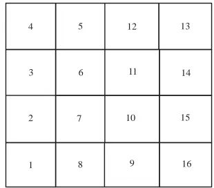
Mathematical model of the MFLP was focused on in this study and the details of the problem are as follows: the MFLP layout problem pattern: it divides the plant site into many rectangular blocks call them template, each template has the same area and shape and each template is assigned to a facility. If the facilities have unequal areas, they could occupy templates and modeled into a cell. Figure 1 which is the example of 6 facilities with 16 templates. If the facilities have equal areas, the problem likes QAP. (Fig. 2) The arrangement by sweeping is to be applied in to the locate department. Measuring distance between each department will be measured in rectilinear from the centroid.
Indices, notation and parameter:
i : The index of a facility where i = 1, 2, 3…N j : The index of a facility where j = 1, 2, 3…N l : The index of a location of template where l = 1,
2, 3…L
: The total vertical and horizontal distance
i, j
d
between facility i and j
: The vertical distance between facility i and j
v ij
d
: The horizontal distance between facility i and j
h ij
d
: The vertical material transportation cost per unit
v
C
: The horizontal material transportation cost per
h
C
unit
: The total templates
A
: The total templates of facility i
i
a
: The material flow between facility i and j
ij
f
: The distance between facility i and j with
e1 ij
d
elevator 1
: The distance between facility i and j with
e2 ij
d
elevator 2
: The coordinator of the centroid of facility i
i i
x , y
: The coordinator of the elevator 1
e1, e1
x y
: The coordinator of the elevator 2
e2, e2
x y
: The floor no. of the facility i
i
Z
: The height between floors
[image:3.612.353.509.93.232.2]H
Fig. 1: The example of 6 facilities with 16 templates
Fig. 2: The example of QAP 16 facilities Decision variable:
(1)
i, l, k
1if facility i assigned to location l and floor No. k U
0 otherwise
(2)
ik
1if facility i assigned tofloor No. k Z
0otherwise
(3)
ij
1if faility i assigned to the same floor with the facility j Z
0 otherwise
Objective function: The objective of the problem in this research is the minimization of the material transporting cost which show in Eq. 4 :
(4)
N 1 N v h
ij v ij h ij i 1 j i+1
Min
f C d +C dSubject to:
(5)
N i i 1a A, i
(6)
i j i j ij e1 e 2 ij ij ij |x x | |y y |;z 1 hij Min d ,d ;z 0
d
(7)
e1
ij i e1 i e1 j e1 i e1
[image:3.612.344.499.268.404.2]Start
Initial vector
Mutation
Crossover or recombination
Fitness evaluation
Selection
Loop repeat
Optimal result
End Yes No
(8)
e2
ij i e2 i e2 j e2 i e2
d | x x | +|y y | | x x | |y y |
(9)
v
ij j i
d H | Z Z |
(10)
h v
ij ij ij
d d d
Constraints:
(11)
total
A A
(12)
K L
ilk i, k 1 l 1U a i
(13)
N L K
ilk total i 1 l 1 k 1U A
(14)
K ik k 1Z 1, i
(15)
N
i ik k i 1a Z A , k
Equation 4, represent an objective function of the model to minimize the material transporting cost. Equation 5 is ensure that total templates are enough for all facilities. Equation 6 is the calculation of horizontal distances between facility i to j. Equation 7 and 8 is the calculation of horizontal distances between facility i to j using elevator No. 1 and 2, respectively. Equation 9 is the calculation of vertical distances between facility i to j. Equation 10 is the total distance between the facility i to j. Equation 11 is ensure that the total space is enough for all facility. Equation 12 is ensures that a plan for all facilities according to the requirement areas of each facility. Equation 13 is a restriction to prevent redundant use of the facility’s area. Equation 14 is restrictions to prevent having the same facility on separate floors. Finally, Eq. 15 is the limitation of the use of space in each floor.
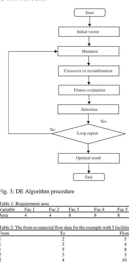
Differential evolution algorithm: The procedures of differential evolution algorithm consist of several steps: create a set of initial vectors, perform a mutation process, cross over or recombination process, fitness evaluation process and selection process. The procedure application is shown in (Fig. 3).
Procedure of MFLP by using differential evolution algorithm: The procedure of MFLP uses the DE algorithm. The values used in the calculation must be set. The variable are as follows: G = round, NP = Numbers of Population, F = Scaling factor and CR = Crossover Rate. In this example calculation, these variables were set as NP = 5, F = 2 and CR = 0.8.
[image:4.612.317.536.81.524.2]Calculation using the DE/rand/1/bin: For example, the problem is two floors with 5 facilities which have the
[image:4.612.75.301.97.315.2]Fig. 3: DE Algorithm procedure
Table 1: Requirement area
Variable Fac.1 Fac.2 Fac.3 Fac.4 Fac.5
Area 4 4 8 8 8
Table 2: The from-to material flow data for the example with 5 facilities
From To Flow
1 2 5
1 3 4
1 5 8
2 3 3
2 4 10
2 5 3
3 4 3
3 5 6
4 5 7
requirement areas in Table 1. The template size is 1 square distance unit and the inter floor distance is 5.0 distance units, material transportation horizontal cost and vertical cost are $1 and $5 per unit per distance, respectively. The material flow is in the Table 2.
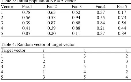
Initial population with a randomized real number between 0 and 1 for each facility (Table 3) which will be used further in mutation and crossover.
Mutation in this step, a position of the vector is randomized (Table 4) and mutated to obtain new solutions that differ from the initial population number by targeting the mutation. The calculation for the mutant vector
(Vi, j, G) is shown in Eq. 16 and an example of a mutation
Table 3: Initial population NP = 5 vector
Vector Fac.1 Fac.2 Fac.3 Fac.4 Fac.5
1 0.78 0.63 0.52 0.37 0.17
2 0.56 0.53 0.94 0.55 0.73
3 0.39 0.87 0.68 0.84 0.56
4 0.41 0.39 0.88 0.21 0.44
5 0.87 0.20 0.11 0.37 0.89
Table 4: Random vector of target vector
Target vector r1 r2 r3
1 1 3 2
2 2 1 3
3 2 5 1
4 1 4 2
[image:5.612.313.541.187.259.2]5 3 5 4
Table 5: Results of mutation in target vector 1 by using DE/rand/1 (F = 2)
Facility 1 2 3 4 5
Xr1=Vector1 (1) 0.78 0.63 0.52 0.37 0.17 Xr2=Vector3 (2) 0.39 0.87 0.68 0.84 0.56 Xr3=Vector2 (3) 0.56 0.53 0.94 0.55 0.73
(1)–(2) (4) 0.39 -0.24 -0.16 -0.47 -0.39
Fx(4):2x (4) (5) 0.78 -0.48 -0.32 -0.94 -0.78 Mutant Vector:(3)+(5) 1.34 0.05 0.62 -0.39 -0.05
Table 6: Results of binomial crossover in vector 1 by DE/rand/1/bin (CR = 0.8)
Facility 1 2 3 4 5
Randb (j) 0.50 0.69 0.98 0.19 0.47
Target vector 0.78 0.63 0.52 0.37 0.17
Mutant vector 1.34 0.05 0.62 -0.39 -0.05
Trial vector 1.34 0.05 0.52 -0.39 -0.05
(16)
i, j,G r3,G r1,G r 2,G
V X F X X
Where:
: Mutant vector
i, j,G
V
: Random vector
r1, G r2, G r3, G
X , X , X
F : Scaling factor (Real number between 0-2)
Crossover or recombination. The vector positions are exchanged in this step, new vectors are generated. The trial vector (Uji, G) is formulated and the trial vectors are
compare and exchanges as in Eq. 17 which is the binomial crossover and an example of a crossover is illustrated in Table 6:
(17)
i , j, k i , j, kV if rand b j CR or j rnbr i i, j,G V if rand b j CR or j rnbr i
U
Where:
Vi, j, G : Mutant Vector
Xi, j, G : Target vector
CR : Crossover constant (real number in the range 0-1) Fitness evaluation. It is the transformation of the vector to get the answer by decoding the vector. The
Table 7: Results of fitness evaluation in vector 1 by DE/rand/1/bin Order of the layout
---
Vector 1 2 3 4 5 Fitness
1 Fac.4 Fac. 5 Fac. 2 Fac. 3 Fac.1 974
-0.39 -0.05 0.05 0.52 1.34
Table 8: Comparison the fitness value in selection process. (DE/rand/1/bin)
Sequence of arrangement
---Vector 1 1 2 3 4 5 Fitness
Trial vector Fac.4 Fac.5 Fac. 2 Fac.3 Fac.1 974 -0.39 -0.05 0.05 0.52 1.34 Target vector Fac.5 Fac.4 Fac.3 Fac.2 Fac.1 991
[image:5.612.71.297.265.334.2]0.17 0.37 0.52 0.63 0.78
Table 9: The example of the selection process for the next generation
Vector 1 2 3 4 5 Fitness
[image:5.612.314.540.281.392.2]1 Target vector 0.78 0.63 0.52 0.37 0.17 991 Trial vector 1.34 0.05 0.52 -0.39 -0.05 974 2 Target vector 0.56 0.53 0.94 0.55 0.73 933 Trial vector -0.05 0.53 1.52 1.20 1.68 922 3 Target vector 0.39 0.87 0.68 0.84 0.56 1058 Trial vector 0.16 0.87 2.18 0.84 0.56 995 4 Target vector 0.41 0.39 0.88 0.21 0.44 747 Trial vector 0.41 1.01 0.22 0.87 0.44 1042 5 Target vector 0.87 0.20 0.11 0.37 0.89 1054 Trial vector -0.55 1.73 0.11 1.15 0.89 1038
Table 10: The vectors are selected for the next generation
Vector 1 2 3 4 5 Fitness
1 1.34 0.05 0.52 -0.39 -0.05 974
2 -0.05 0.53 1.52 1.20 1.68 922
3 0.16 0.87 2.18 0.84 0.56 995
4 0.41 0.39 0.88 0.21 0.44 747
5 -0.55 1.73 0.11 1.15 0.89 1038
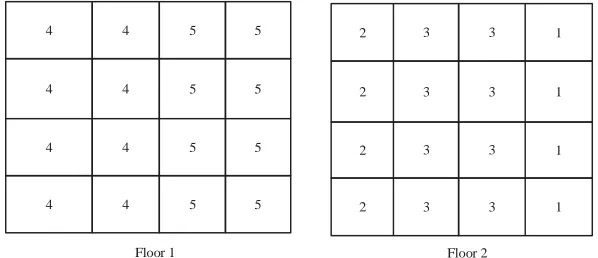
method used to decode the vector is the order Ranking Value method (ROV) which is arranged from ascending values. Then the order will be used to find the answer and arrange the facility that corresponds to the order of the vector and calculate the fitness from the objective function Eq. 4. The results of the fitness evaluation of DE/rand/1/bin is illustrated in Table 7.
The fitness value was calculating from Eq. 4, the result of facility layout as show in Fig. 4 which arrangement by sweeping from the left corner template down to lower.
[image:5.612.316.540.412.471.2]4 4 5 5
4 4 5 5
4 4 5 5
4 4 5 5
2
2
2
2 3
3
3
3 3
3
3
3 1
1
1
1
[image:6.612.158.457.96.225.2]Floor 1 Floor 2
Fig. 4: The result of facility layout from vector 1
(18)
i , j, G i , j, G i , j, G i , j, GU if f U f X i, j,G 1 X otherwise
X
Where:
: Trial vector
i, j,G
U
: Target vector in the next generation
i, j,G 1
X
Calculation using the DE/rand/2/bin: DE/rand/2/bin and DE/rand/2/exp have step similar to DE/rand/1/bin and DE/rand/1/exp but have different calculations in mutation step as Eq. 19:
(19)
i, j,G r5,i,G r1,i,G r 2,i,G r 3,i,G r 4,i,G
V X F X X X X
RESULTS AND DISCUSSION
Analysis of the results from the experiment on DE for solving MFLP: Solving MFLP applies a VBA program running on a laptop, Core i5, 2.5 GHz, 12 GB RAM, Windows 10 operating system. It calculates and shows the result and the layout on spreadsheet.
In the experiment, the problem of 11 and 21 facilities, respectively which have detail in Appendix A using 3 levels of F parameters, factors were F = 0.9, 1.5 and 2 and 4 levels of CR. The factors were CR = 0.2, 0.4, 0.6 and 0.8 which were tested with 4 DE algorithm as follows: DE/rand/1/bin, DE/rand/2/bin, DE/rand/1/exp and DE/rand/ 2/exp.
F (Scaling factor) parameter: In this experiment, F is divided into 3 levels which are 0.9, 1.5 and 2, respectively for the problem 11A (11 facilities) and 21A (21 facilities) CR = 0.8, NP = 50, G = 300. The results show in Table 11.
CR (Crossover Rate) parameter: The experiment using CR, divided into 4 levels which are 0.2, 0.4, 0.6 and 0.8, respectively with the problem 11 A (11 facilities) and 21A (21 facilities), F = 2, NP = 50 and G = 300. The results show in Table 12.
From the experimental results for parameter determination, it can be seen that DE/rand/1/bin and DE/rand/2/bin were the method that give the better value than DE/rand/1/exp and DE/rand/2/exp. For F parameter, F = 0.9 is suitable for 11 facilities problem or medium problems, F = 2.0 is suitable for 21 facilities problem or large problems. CR = 0.8 gives the answer as a good average fitness. Therefore, in the next chapter will set F = 0.9 for 11 and 12 facilities problem and F = 2 for 21 facilities problem and CR = 0.8 for all problems.
The results from the comparison of DE Algorithm and the other methods: Table 13. The results of using the basic DE algorithm compared with using the MULTIPLE, SABLE and best soln. in MFLP benchmark problems with Meller’s problems.
The benchmark problems of MULTIPLE and SABLE methods on problem 11-1, 11-2, 12, 21-1, 21-2 and 21-3 with Meller’s problems. The result of the experiment on the MFLP by using the basic DE algorithm consisted of two methods as follows: DE/rand/1/bin and 2/bin. The cost of material transportation and the% of comparison with the best solution from Meller and Bozer (1997) are in the Table 13. The comparison of maximum calculation time in seconds is depicted in Table 14. Table 13 shows that two method of basic DE can generate the optimal solutions better than multiple for all problems and found four problems (11-1, 21-1, 21-2 and 21-3) that DE/rand/2/bin generate the optimal solutions better than SABLE. The problems, especially, 21-3 is approximately 21.7-22.3% comparison with the best solution.
Table 11: The results of the experimental using 4 DE algorithm with different F values
Problem F-values DE/rand/1/bin cost($) DE/rand/2/bin cost ($) DE/rand/1/exp cost($) DE/rand/2/exp cost($)
11A 0.9 8078.25 8086.93 8148.49 8143.25
1.5 8085.21 8092.60 8312.36 8131.44
2 8085.96 8096.21 8291.12 8149.51
21A 0.9 15186.39 15540.09 20160.90 18843.96
1.5 15325.23 15789.74 21149.53 19572.93
[image:7.612.71.541.190.276.2]2 14812.13 15481.70 21226.85 19546.60
Table 12: The results of the experiment on MFLP by using 4 DE algorithm with different CR values
Problem CR DE/rand/1/bin cost ($) DE/rand/2/bin cost ($) DE/rand/1/exp cost ($) DE/rand/2/exp cost ($)
11A 0.2 8086.66 8084.76 9385.78 9671.60
0.4 8070.00 8068.10 8884.49 8650.66
0.6 8075.26 8077.71 8562.93 8256.24
0.8 8068.98 7894.24 8291.12 8149.51
21A 0.2 16719.80 16566.00 25812.00 26669.90
0.4 16931.30 15822.40 26913.70 24349.60
0.6 16025.60 15657.00 24884.10 22933.80
0.8 14323.40 14964.90 21732.00 19016.20
Table 13: The cost of material transportation and percentage of comparison with SABLE, MULTIPLE and best solution form Meller and Bozer
MULTIPLE SABLE DE/rand/1/bin DE/rand/2/bin
--- --- ---
---Problem Comparison Comparison Comparison Comparison
(floor) Best Soln* Cost ($) with best Soln (%) Cost ($) with best Soln (%) Cost ($) with best Soln (%) Cost ($) with best Soln (%)
11-1 (2) 8275.7 16702 101.8 8477 2.4 7990.0 -3.5 7967.5 -3.7
11-2 (2) 2493.9 2910 16.7 2493.9 0 2542.5 1.9 2527.18 1.3
12 (3) 1513.1 2153 42.3 1513.1 0 1810.95 19.7 1810.95 19.7
21-1 (4) 14970 18553 23.9 14970 0 14302.0 -4.5 13254.0 -11.5
21-2 (4) 11854.7 14410 21.6 11854.7 0 12478.0 5.3 11841.3 -0.1
21-3 (4) 10263.5 11787 14.8 10263.5 0 7973.67 -22.3 8032.0 -21.7
*Meller (1992)
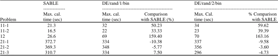
Table 14: The maximum calculation time comparison benchmark problems
SABLE DE/rand/1/bin DE/rand/2/bin
--- ---
---Max. cal. Max. cal. Comparison Max. Cal. % Comparison
Problem time (sec) time (sec) with SABLE (%) time (sec) with SABLE
11-1 21.3 32 50.23 34 59.62
11-2 16.5 22 33.33 23 39.39
12 26.6 69 159.40 70 163.16
21-1 372.7 334 -10.38 337 -9.58
21-2 369.3 348 -5.77 356 -3.60
21-3 310.7 334 7.50 296 -4.73
CONCLUSION
Next is conclusive findings of the research on solving the multi-floor facility layout problem by differential evolution algorithm, two DE algorithm generate the better solution more than multiple for all problems. DE/rand/2/bin produce better solution when compared to the best solution on Problems 11-1, 21-1, 21-2 and 21-3 which calculate the comparison in percentage are 3.7, 11.5, 0.1 and 21.7%, respectively. DE/rand/1/bin produced better solution when compared to the best solution on problems 11-1, 21-1 and 21-3 which calculate the comparison in percentage are 3.5, 4.5 and 22.3%, respectively.
With regard to the maximum calculation time, DE method take the maximum calculation time less than the maximum calculation time of sable on the 21 facilities problems. About (21-1, 21-2, 21-3) very high maximum
calculation time caused by programming calculations. Using the VBA programming is a calculation and display through the spread sheet to show the facility layout making the calculation time slower. When compared to the programming calculated from high level languages such as C language etc. Hence, when choosing a program for processing, the program should be selected appropriately. For accuracy of comparison of experimental results.
[image:7.612.69.544.293.389.2] [image:7.612.71.540.416.511.2]Elevator Fixed facility
Floor 2
Floor 1
11 11
11 11
11 11
Elevator Fixed facility
Floor 2-4
Floor 1 21
21
21
21
21
21
21
21
ACKNOWLEDGEMENTS
We would like to thank Industrial Engineering Department, Faculty of Engineering, Ubon Ratchathani University and my family, teachers, staffs and friends for their support and encouragement.
APPENDIX A
Problem 11A: The areas of each facility are shown in Table A-1 with the from-to flow values as shown in Table A-2. The cost of material handling is $1 and $5 per unit of horizontal and vertical distances, respectively. The template size is 2.5 square distance units and the inter floor distance is 10 distance units. Figure A-1 also indicates the location of two elevators and the fixed facility location.
Table A-1: The facility area for problem 11A
Facility 1 2 3 4 5 6 7 8 9 10 11
Area 3 2 4 5 2 3 4 5 1 1 6
(Templates)
Table A-2: The from-to flow values for problem 11A
From To Flow From To Flow
1 2 10 5 7 40
1 5 140 5 10 20
1 6 90 6 3 10
1 7 20 6 9 20
1 9 40 7 8 10
2 3 10 8 11 10
3 4 10 9 10 20
4 11 4 10 11 20
5 2 10 11 1 146
Fig. A-1: The elevator location and fixed facility location for problem 11A
Problem 21A: The areas of each facility are shown in Table A-3 with the from-to flow values as shown in Table A-4. The cost of material handling is $1 and $5 per unit of horizontal and vertical distances, respectively. The template size is 4.0 square distance units and the inter floor distance is 2.5 distance units. Figure A-2 also indicates the location of two elevators and the fixed facility location.
Table A-3: The facility area for problem 21A
Facility Area (Template) Facility Area (Template)
1 2 12 2
2 1 13 2
3 2 14 1
4 2 15 1
5 4 16 2
6 2 17 2
7 4 18 4
8 2 19 2
9 2 20 2
10 2 21 8
11 1
Table A-4: The from-to flow values for problem 21A
From To Flow From To Flow
1 2 115 3 11 10
1 21 112 3 16 80
2 3 10 3 20 20
2 12 20 4 5 10
2 13 50 4 7 40
2 14 80 4 8 100
2 19 20 4 15 8
3 4 100 4 17 100
3 5 200 5 10 4
3 6 20 5 18 60
3 9 100 6 10 2
REFERENCES
Abdinnour-Helm, S. and S.W. Hadley, 2000. Tabu search based heuristics for multi-floor facility layout. Int. J. Prod. Res., 38: 365-383
Afrazeh, A., A. Keivani and L.N. Farahani, 2010. A new model for dynamic multi floor facility layout problem. Adv. Model. Optim., 12: 249-256. Ahmadi, A. and M.R.A. Jokar, 2016. An efficient
multiple-stage mathematical programming method for advanced single and multi-floor facility layout problems. Applied Math. Modell., 40: 5605-5620. Berntsson, J. and M. Tang, 2004. A slicing structure
representation for the multi-layer floorplan layout problem. Proceedings of the Workshops on Applications of Evolutionary Computation, April 5-7, 2004, Springer, Berlin, Germany, pp: 188-197. Bozer, Y.A., R.D. Meller and S.J. Erlebacher, 1994. An improvement-type layout algorithm for single and multiple-floor facilities. Manage. Sci., 40: 918-932. Cao, E. and M. Lai, 2010. The open vehicle routing problem with fuzzy demands. Expert Syst. Appl., 37: 2405-2411.
Chang, C.H., J.L. Lin and H.J. Lin, 2006. Multiple-floor facility layout design with aisle construction. Ind. Eng. Manage. Syst., Vol. 5,
Donaghey, C.E. and V.F. Pire, 1990. Solving the facility layout problem with BLOCPLAN. Industrial Engineering Department, University of Houston, Houston, Texas.
Ganokgarn, J., P. Rapeepan and M. Paroon, 2015. Solving an simple assembly line balancing problem by differential evolution: A case study of garment industry. Princes Naradhiwas Univ. J., 7: 153-164. Georgiadis, M.C., G.E. Rotstein and S. Macchietto, 1997.
Optimal layout design in multipurpose batch plants. Ind. Eng. Chem. Res., 36: 4852-4863.
Ha, J.K. and E.S. Lee, 2016. Development of an optimal multifloor layout model for the generic liquefied natural gas liquefaction process. Korean J. Chem. Eng., 33: 755-763.
Hahn, P.M., J.M. Smith and Y.R. Zhu, 2010. The muti-story space assignment problem. Ann. Oper. Res., 179: 77-103.
Huang, C., C.K. Wong and C.M. Tam, 2010. Optimization of material hoisting operations and storage locations in multi-storey building construction by mixed-integer programming. Automation Construc., 19: 656-663.
Irohara, T. and M. Goetschalckx, 2007. Decomposition solution algorithms for the multi-floor facility layout problem with elevators. Proceedings of the 19th International Conference on Production Research (ICPR), July 29-August 2, 2007, Valparaiso, Chile, PP: 1-6.
Izadinia, N. and K. Eshghi, 2016. A robust mathematical model and ACO solution for multi-floor discrete layout problem with uncertain locations and demands. Comput. Ind. Eng., 96: 237-248.
Johnson, R.V., 1982. Spacecraft for multi-floor layout planning. Manage. Sci., 28: 407-417.
Kaku, B.K., G.L. Thompson and I. Baybars, 1988. A heuristic method for the multi-story layout problem. Eur. J. Oper. Res., 37: 384-397.
Kia, R., F. Khaksar-Haghani, N. Javadian and R. Tavakkoli-Moghaddam, 2014. Solving a multi-floor layout design model of a dynamic cellular manufacturing system by an efficient genetic algorithm. J. Manuf. Syst., 33: 218-232.
Kochhar, J.S. and S.S. Heragu, 1999. Facility layout design in a changing environment. Int. J. Prod. Res., 37: 2429-2446.
Kochhar, J.S., 1998. MULTI-HOPE: A tool for multiple floor layout problems. Intl. J. Prod. Res., 36: 3421-3435.
Krishnan, K.K., A.A. Jaafari, M. Abolhasanpour and H. Hojabri, 2009. A mixed integer programming formulation for multi-floor layout. Afr. J. Bus. Manage., 3: 616-620.
Lee, K.Y., M.I. Roh and H.S. Jeong, 2005. An improved genetic algorithm for multi-floor facility layout problems having inner structure walls and passages. Comput. Oper. Res., 32: 879-899.
Matsuzaki, K., T. Irohara and K. Yoshimoto, 1999. Heuristic algorithm to solve the multi-floor layout problem with the consideration of elevator utilization. Comput. Ind. Eng., 36: 487-502. Meller, R.D. and Y.A. Bozer, 1996. A new simulated
annealing algorithm for the facility layout problem. Int. J. Prod. Res., 34: 1675-1692.
Meller, R.D. and Y.A. Bozer, 1997. Alternative approaches to solve the multi-floor facility layout problem. J. Manuf. Syst., 16: 192-203.
Meller, R.D., 1992. Layout algorithms for single and multiple floor facilities. Ph.D Thesis, University of Michigan, Ann Arbor, Michigan.
Patsiatzis, D.I. and L.G. Papageorgiou, 2002. Optimal multi-floor process plant layout. Comput. Chem. Eng., 26: 575-583.
Seehof, J.M. and W.O. Evans, 1967. Automated layout design program. J. Ind. Eng., 18: 690-695.
Singh, S.P. and R.R.K. Sharma, 2006. A review of different approaches to the facility layout problems. Int. J. Adv. Manuf. Technol., 30: 425-433.
Sresracoo, P., N. Kriengkorakot, P. Kriengkorakot and K. Chantarasamai, 2018. U-shaped assembly line balancing by using differential evolution algorithm. Math. Comput. Appl., Vol. 23,