University of Warwick institutional repository:
http://go.warwick.ac.uk/wrap
A Thesis Submitted for the Degree of PhD at the University of Warwick
http://go.warwick.ac.uk/wrap/57056
This thesis is made available online and is protected by original copyright.
Please scroll down to view the document itself.
AUTHOR:Quentin Caudron DEGREE:Ph.D.
TITLE:Neuronal Computation on Complex Dendritic Morphologies
DATE OF DEPOSIT: . . . .
I agree that this thesis shall be available in accordance with the regulations governing the University of Warwick theses.
I agree that the summary of this thesis may be submitted for publication. I agree that the thesis may be photocopied (single copies for study purposes only).
Theses with no restriction on photocopying will also be made available to the British Library for microfilming. The British Library may supply copies to individuals or libraries. subject to a statement from them that the copy is supplied for non-publishing purposes. All copies supplied by the British Library will carry the following statement:
“Attention is drawn to the fact that the copyright of this thesis rests with its author. This copy of the thesis has been supplied on the condition that anyone who consults it is understood to recognise that its copyright rests with its author and that no quotation from the thesis and no information derived from it may be published without the author’s written consent.”
AUTHOR’S SIGNATURE: . . . .
USER’S DECLARATION
1. I undertake not to quote or make use of any information from this thesis without making acknowledgement to the author.
2. I further undertake to allow no-one else to use this thesis while it is in my care.
DATE SIGNATURE ADDRESS
. . . .
. . . .
. . . .
. . . .
Neuronal Computation on
Complex Dendritic Morphologies
by
Quentin Caudron
Thesis
Submitted to the University of Warwick
for the degree of
Doctor of Philosophy
Centre for Complexity Science
Contents
Acknowledgements v
Declarations vi
Abstract vii
Chapter 1 Preface 1
1.1 The Brain in Context . . . 1
1.2 Thesis Outline . . . 3
Chapter 2 Of Neurons and Dendrites 5 2.1 A Brief History of Neuroscience . . . 5
2.2 Morphology of Neurons . . . 7
2.2.1 Soma . . . 9
2.2.2 Axon . . . 10
2.2.3 Dendrites . . . 11
2.2.4 Diversity of Dendrites . . . 11
2.3 The Biophysics of Excitable Cells . . . 14
2.3.1 Structure of the Cell Membrane . . . 14
2.3.2 Resting Potential and Equivalent Circuits . . . 16
2.4 Neuronal Communication . . . 19
2.4.1 Action Potentials . . . 19
2.4.2 Synapses . . . 21
2.4.3 Network Connectivity and Structure . . . 23
2.4.4 Plasticity . . . 25
2.5 The History of Dendritic Physiology and Modelling . . . 26
2.6 Dendritic Computation . . . 31
2.6.1 Spatiotemporal Filtering . . . 32
2.6.3 Active Currents . . . 34
2.6.4 Coincidence Detection . . . 35
2.6.5 Directional Selectivity . . . 36
2.6.6 Dendritic Democracy . . . 37
2.6.7 Computing with Dendrites . . . 37
2.7 Continuous-Space Dendritic Modelling . . . 37
2.7.1 Analytical Approaches to Cable Problems . . . 38
2.8 Conclusions . . . 44
Chapter 3 Linear Cable Theory and the Dendritic Path Integral 46 3.1 The Linear Cable Equation . . . 47
3.1.1 A Note on Units . . . 48
3.1.2 Derivation of the Cable Equation . . . 49
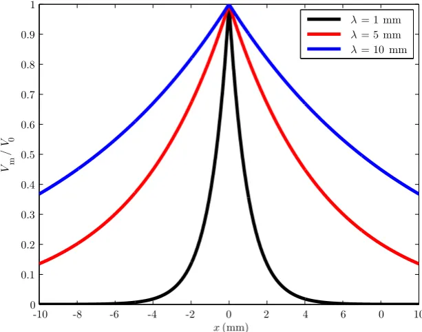
3.1.3 Characteristic Scales . . . 52
3.1.4 Assumptions . . . 55
3.2 A Note on Integral Transforms . . . 57
3.3 Some Concepts in Linear Systems Theory . . . 61
3.4 Steady-State and Time-Dependent Solutions . . . 66
3.4.1 Boundary Conditions for the Single Cable . . . 67
3.4.2 Steady State on a Semi-Infinite Cable . . . 67
3.4.3 Steady State on a Finite Cable with Closed Ends . . . 68
3.4.4 Steady State on a Finite Cable with One Open End . . . 70
3.4.5 General Solution . . . 72
3.4.6 Alpha Currents . . . 77
3.4.7 Rectangular Pulse . . . 79
3.5 The Path Integral for Dendritic Trees . . . 79
3.5.1 Rules for Trip Construction . . . 84
3.5.2 Trip Classes . . . 87
3.5.3 Theoretical Convergence and Term Ordering . . . 87
3.6 Closed-Form Solutions for Simplified Structures . . . 94
3.6.1 Finite Single Cable . . . 94
3.6.2 Star Graph Cells . . . 95
3.7 Conclusions . . . 101
Chapter 4 Time-Domain Methods 103 4.1 Graph Theory and Algorithms Terminology . . . 104
4.2 The Four Classes Algorithm . . . 107
4.3 A Formal Grammar for Paths on Graphs . . . 111
4.3.1 Some Language Theory Terminology . . . 111
4.3.2 The Improved Four Classes Algorithm . . . 112
4.3.3 Application of the Improved Four Classes Algorithm . . . 113
4.4 The Length Priority Algorithm . . . 117
4.5 Monte Carlo Method . . . 119
4.5.1 Random Walkers and Diffusion . . . 119
4.5.2 Random Hoppers . . . 120
4.5.3 Obtaining the Green’s Function Solution . . . 121
4.6 Trip-Grouping Matrix Algorithm . . . 123
4.6.1 Discretisation of the Dendritic Tree . . . 124
4.6.2 Construction of the Edge-Adjacency Matrix . . . 125
4.6.3 Computing the Path Integral . . . 127
4.6.4 Example Calculation . . . 128
4.7 Convergence of Time-Domain Methods . . . 130
4.7.1 Morphologies . . . 130
4.7.2 Implementations . . . 132
4.7.3 Validation Against Numerics . . . 133
4.7.4 Error of Convergence . . . 133
4.7.5 Convergence of the Length Priority Methods . . . 135
4.7.6 Convergence of the Monte Carlo Method . . . 138
4.7.7 Convergence of the Trip-Grouping Matrix Algorithm . . . 139
4.7.8 Structural-Electrotonic Properties . . . 140
4.8 Conclusions . . . 145
Chapter 5 Laplace-Domain Methods 147 5.1 Cable Systems in the Laplace Domain . . . 148
5.1.1 Laplace-Domain Solutions . . . 149
5.1.2 Boundary Conditions . . . 149
5.2 Motifs . . . 150
5.2.1 The Motif Concept . . . 150
5.2.2 Edge Orientation . . . 151
5.2.3 Nomenclature : The Set of Motifs . . . 152
5.3 Forward Motif Method . . . 152
5.3.1 Coefficient Expressions . . . 153
5.3.2 Motif Matrix Rows . . . 159
5.4 Conclusions . . . 166
Chapter 6 Discussion 167
Acknowledgements
During my four years at the Centre for Complexity Science at Warwick, I have
learned a great deal about mathematics, science, and research in general. In the
process, established academics would become colleagues, and colleagues would
be-come friends. Without their aid, support, and encouragement, I would simply not
be where I am today.
First amongst these is my supervisor, Dr. Yulia Timofeeva, who always
guided me with patience and knowledge, while letting me explore the landscape
in my own way. Her expertise and advice have led me to produce work of which I
am genuinely proud, and for this, I am extremely grateful.
To the talented graph theorist and mathematician, Simon Donnelly, I offer
my deepest gratitude. Discussions with you would always bear fruit, the end result
of which is evident in this thesis.
I wish to thank the extremely talented mathematicians, Jamie Harris and
Sam Brand, for many discussions spent poring over blackboards.
My family remain a neverending source of support and motivation. To my
wife, Madi, for her love and for my sanity; to my father, for keeping things in
perspective; to my mother, for always being there; and to my siblings, for being
Declarations
The work in this thesis is a presentation of my original research. Every effort has
been made to credit the authors of the peer-reviewed literature which provide the
foundations upon which this work is built, and the collaborators who contributed
their skill and time in the development of this work.
Parts of the work in Chapter 4 were done in collaboration with Simon Donnelly,
of Edinburgh’s Neuroinformatics Doctoral Training Centre, whose help was
funda-mental to my understanding of aspects of graph theory, and subsequently to my
development of these algorithms; and Sam Brand, of Warwick Complexity, who
in-troduced me to the Feynman-Kac relation between some differential equations and
stochastic processes. This work has been published in the Journal of Mathematical
Neuroscience, as
Q. Caudron, S. R. Donnelly, S. P. C. Brand, and Y. Timofeeva,
Computational convergence of the path integral for real dendritic morphologies,
The Journal of Mathematical Neuroscience, 2 (11), 2012.
The Motif method presented in Chapter 5 was developed in collaboration with Jamie
Harris, of Warwick Complexity, whose insight and experience with Green’s functions
brought us to the idea of motifs on trees.
Abstract
When we think about neural cells, we immediately recall the wealth of
elec-trical behaviour which, eventually, brings about consciousness. Hidden deep in the
frequencies and timings of action potentials, in subthreshold oscillations, and in
the cooperation of tens of billions of neurons, are synchronicities and emergent
be-haviours that result in high-level, system-wide properties such as thought and
cogni-tion. However, neurons are even more remarkable for their elaborate morphologies,
unique among biological cells. The principal, and most striking, component of
neu-ronal morphologies is the dendritic tree.
Despite comprising the vast majority of the surface area and volume of a
neuron, dendrites are often neglected in many neuron models, due to their sheer
complexity. The vast array of dendritic geometries, combined with heterogeneous
properties of the cell membrane, continue to challenge scientists in predicting
neu-ronal input-output relationships, even in the case of subthreshold dendritic currents.
In this thesis, we will explore the properties of neuronal dendritic trees, and
how they filter and integrate the electrical signals that diffuse along them. After
an introduction to neural cell biology and membrane biophysics, we will review
Abbott’s dendritic path integral in detail, and derive the theoretical convergence
of its infinite sum solution. On certain symmetric structures, closed-form solutions
will be found; for arbitrary geometries, we will propose algorithms using various
heuristics for constructing the solution, and assess their computational convergences
on real neuronal morphologies. We will demonstrate how generating terms for the
a computationally-significant number of terms is required for reasonable accuracy.
We will, however, derive a highly-efficient and accurate algorithm for application to
discretised dendritic trees. Finally, a modular method for constructing a solution in
Chapter 1
Preface
“
It is the brain which is the messenger to the understanding.”
- Hippocrates1.1
The Brain in Context
running on some of the world’s most powerful computers, the project’s predeces-sor, the Blue Brain Project [Markram, 2006], had simulated a cortical column of ten thousand neurons in 2008, and a mesocircuit of only one million neurons by 2011 – a small fraction of the human brain’s nearly 1011neurons [Herculano-Houzel, 2009].
In contrast, models focusing on simplification of the biological processes in favour of mathematical efficiency are able to simulate far larger systems. These ap-proaches abstract away the biological detail, using functional forms to approximate the system’s dynamics instead of fully simulating the system. This is exemplified by Izhikevich’s 2005 simulation, in which a system of 1011neurons and 1015synapses –
a system the size of a full human brain – was simulated on the neuronal level, albeit in far less detail than with biophysical models. The simulation ran over fifty days, and provided one second of real data. Izhikevich and Edelman’s [2008] later sim-ulation later reconciled the single neuron, cortical columnar, and large-scale white matter spatial scales, informed by experimental data; due to the added complexity, this system only contained one million neurons.
One element brought into Izhikevich’s 2008 simulation which was absent from his earlier, larger system, was branching dendritic morphology. The inclusion of spatially-extended dendritic cables introduces a significant computational diffi-culty : due to their arbitrarily-branching natures, electrical activity on dendritic trees cannot be solved for explicitly, except in very rare cases. As such, dendrites are typically modelled discretely in space, and the voltage across their membranes computed numerically, which can be very slow.
expressions requiring numerical inversion from the frequency domain. These results all provide a means of computing the impulse response function of a dendritic sys-tem, providing insight into the dynamics of current flow along the dendritic tree and allowing the efficient computation of the voltage response anywhere on the tree, as a result of current input.
1.2
Thesis Outline
Chapter 2
We begin by a short history of the field of neuroscience, from our knowledge of it in antiquity, and through its major developments in the twentieth century, when neuronal cable theory was born. We then introduce the general biophysics of the neuron, focusing on typical morphology and the excitable properties of its cell mem-brane. We discuss aspects of neuronal communication, including the generation of action potentials, how synapses transmit signals from one neuron to another, and some of the possible methods used by neurons to encode information. After a re-view of the history of dendritic modelling, and of modern literature on methods for approaching dendritic cable problems, we finish with a few brief examples of where dendrites may perform computations.
Chapter 3
After a review of important concepts in integral transforms and linear systems, the linear cable equation is introduced, along with the assumptions made in its deriva-tion, some of its steady-state solutions, and the general time-dependent solution on the infinite cable. We then present a summary of Abbott et al.’s [1991] path integral for dendritic trees, a method for computing the transmembrane voltage on arbitrary branching structures; we discuss rules for constructing the infinite se-ries solution and derive a novel proof of its theoretical convergence, making fewer restrictive assumptions than in the proof provided by Abbott [1992].
Chapter 4
a language-theoretic approach to constructing the terms in the series as an im-provement on the algorithm provided by Cao and Abbott [1993], and then using a
k-shortest paths algorithm for efficient implementation. We compare Cao and Ab-bott’s [1993] Four Classes trip ordering with our Length Priority ordering of terms in assessing the computational convergences of the algorithms. A Monte Carlo method is then developed, ordering trips according to a probabilistic heuristic. Finally, we draw on methods from graph theory to derive an efficient algorithm for grouping trips by discretised lengths in order to construct the series solution using blocked terms.
Chapter 5
The methods and algorithms presented in the previous chapter were approaches to computing the dendritic path integral, a convergent time-domain series solution. Here, we consider the exact solution to cable theory problems in the Laplace domain, by constructing a linear system of equations based on graphical motifs. We derive a forward method which requires the inversion of a motif matrix to obtain the coeffi-cients of the Laplace-domain solution, which is easily computationally-implemented.
Chapter 6
Chapter 2
Of Neurons and Dendrites
“
Most of the brain consists of “wires” [. . .] The connections as a whole define the information content of the system.”
- Campbell [1989]2.1
A Brief History of Neuroscience
The brain is arguably the most complex object in the known universe. At one time thought to be a continuous mesh of tissue, we now know that the human brain contains on the order of one hundred billion neurons. For every neuron, there are ten neuroglia, cells responsible for modulating neurotransmission, amongst other functions. From this enormous, intricately interconnected network of highly-nonlinear units, somehow, emerges consciousness, memory and emotion.
and many others. It was with the invention of the microscope, however, and the pivotal work of Camillo Golgi on hisreazione nera, later named the Golgi stain, that individual neurons were discovered. This brought on the formation of the neural doctrine, proposed by Santiago Ram´on y Cajal, that the brain consists of a large number of individual functional units, called neurons. Experiments pioneered by Luigi Galvani developed our knowledge of excitable tissue such as muscle, and in the late 19th Century, neurons were shown to be electrically excitable and that their
electrical states were correlated with those of their neighbours. As research methods improved, we learned much of structural and functional neuroanatomy, furthered by contributions from scientists such as Broca, Wernicke, and Brodmann.
In 1864, Julius Bernstein developed the differential rheotome, an instrument for the quantitative measurement of the neuronal action potential. Decades later, he proposed the hypothesis that excitable cells are surrounded by a selectively-permeable membrane, and explained excitation as an increased permeability to potassium ions. It was only fifty years later, however, that the first mathemat-ical description of the action potential was published. Work by Ostwald, Cole, Curtis, Katz, and many others, culminated in a series of papers by Alan Hodgkin and Andrew Huxley on a set of nonlinear ordinary differential equations, describing the initiation and propagation of action potentials; this work earned Hodgkin and Huxley the Nobel Prize in Physiology or Medicine in 1963. Today, the Hodgkin-Huxley model – and related conductance-based neural models - are still extensively used in the modelling and simulation of networks of neurons where biophysical re-alism is required. Less realistic, the simplest model neuron is arguably Lapicque’s integrate-and-fire cell, describing neurons as a simple capacitor circuit. Appreci-ated for its mathematical and computational simplicity, it has also spawned many variants, such as the leaky integrate-and-fire, as well as nonlinear (quadratic, expo-nential, adaptive) versions.
neuronal structure can be calculated or simulated using one of many approaches derived from Rall’s models and methods, with cable theory at their heart.
Passive cable theory, the linear framework adapted to dendrites by Rall, allows mathematically-tractable insight to be made regarding the dendrites’ spa-tiotemporal filtration properties on signal integration. It provides a means to tackle cable problems for large, complex structures, such as those representative of neu-ronal morphology, enabling us to replicate or explain experimentally-verified find-ings. Cable theory models the continuum flow of ions along one-dimensional cables, according to a set of assumptions regarding the typical dimensions, chemical com-position, and electrical properties, of dendritic fibres.
Cable theory provides us with the ability to compute the spatiotemporal filtering properties of a tree’s morphology. This fundamental characteristic can provide a great deal of information regarding how a particular neuron integrates electric currents : the impulse response function, which encodes the system’s reaction to an external stimulus, can tell us the amount of delay or attenuation that a signal will incur as it diffuses along the dendritic cables. It can aid us in understanding how a number of signals from different parts of a dendritic tree are integrated and filtered when they reach the soma. Due to this signal filtration, understanding the link between dendritic morphology and the signals observed at the soma as a response to stimulus is essential in the study of neuronal input-output relations.
The manner in which the brain processes information remains a mystery. In the past, simple computations were attributed to individual neurons; it was assumed that a network as complex as the brain could produce significant emergent behaviour, accounting for higher levels of information processing, from perception to emotion. Incoming signals would be summed, or integrated, and if a threshold was met, the neuron would fire a spike. By adding dendrites into this picture, we immediately have available a larger number of computational tools, from nonlinear summation in active dendrites, to resonance, to delay and linear signal filtration in passive dendrites [Sprustonet al., 1999]. Today, we understand the importance of dendrites in neuronal computations and the additional dynamics they bring to communication in the brain. There is therefore a great deal of information to be found in a neuron’s morphology.
2.2
Morphology of Neurons
highly-specialised cells process and transmit information between one another and to the rest of the body, via a complex and elaborate branching network of filamentous neu-ral processes, the axons and dendrites. The human brain, approximately 1200 cm3
in volume [Cosgroveet al., 2007] and weighing 1.5 kg [Parent and Carpenter, 1995], contains on the order of 1011 individual neurons [Herculano-Houzel, 2009], each
with an average of 104 connections to other neurons [Drachman, 2005], local or
dis-tal, forming anything from small, sparse clusters to enormous, densely-connected hypercolumns.
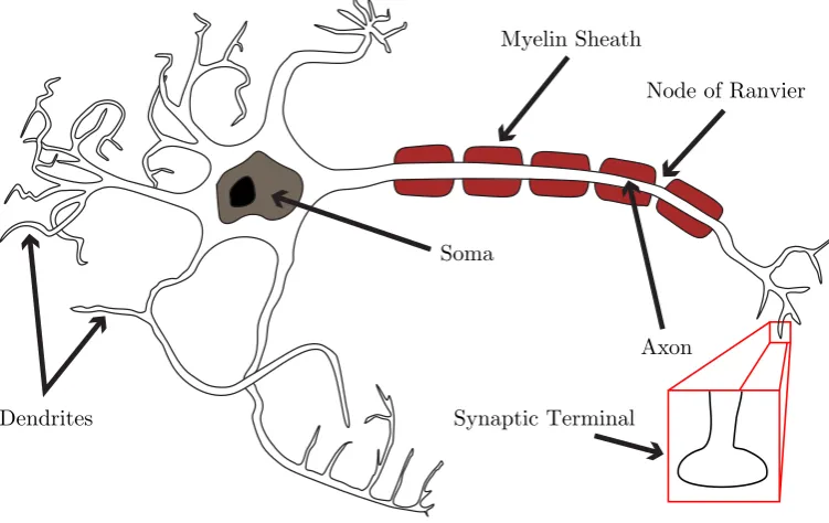
Myelin Sheath
Dendrites
Axon Soma
Node of Ranvier
[image:20.595.135.511.254.491.2]Synaptic Terminal
Figure 2.1: A caricatured neuron, showing the key components of neuronal structure and morphology.
of a neuron, demonstrating the three parts that generally make up a neuron : the soma, the axon, and the dendrites.
2.2.1 Soma
[image:21.595.162.480.296.537.2]Neuronal cell bodies exhibit a great variety of sizes. Some of the largest known somas belong to the sea slugAplysia california, and can approach close to 1 mm in diameter [Gillette, 1991] – although they are usually much more compact. The soma houses a large number of organelles, such as the nucleus and Nissl granules, which are important sites for protein synthesis, particularly the synthesis of neurotransmitters. Other synthesis also largely occurs inside the soma : the sugars and lipids that make up the intracellular fluid, or cytoplasm, are made here.
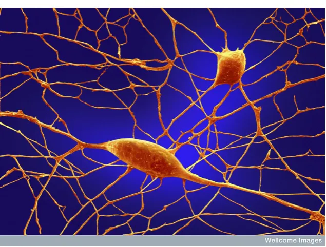
Figure 2.2: Scanning electron micrograph of differentiating Purkinje neu-rons. Once their development is complete, these neurons will become some of the largest in the brain. Annie Cavanagh, Wellcome Library, London.
2.2.2 Axon
The axon is a long projection that can extend great distances, generally branching extensively as it meets other neighbouring (or distal) neurons. It connects to the cell body at the axon hillock, a specialised part of the soma that swells to become the axon. Its high density of ion channels makes it capable of generating action potentials, which then propagate down the axon, away from the soma, usually to other neurons but also to muscle or gland cells. Axons are typically wrapped in myelin sheaths, composed of an electrically-insulating material which reduces mem-brane capacitance while increasing its resistance, leading to a smaller loss of current through the membrane. The small spaces between the myelin sheaths, the nodes of Ranvier (see Figure 2.1), reveal the uninsulated axonal membrane, which is capable of high levels of electrical activity. The action potential is continuously regenerated at these points, where electrical signals are amplified by the triggering of further ac-tion potentials. Hence, the axon supports the faster saltatory propagaac-tion of acac-tion potentials.
Figure 2.3: Confocal micrograph of aDrosophila neuron growing in vitro. The axon can be seen emerging from the soma at the axon hillock, retaining a fairly constant diameter as it branches into smaller protrusions. Guy Tear, Wellcome Library, London.
2.2.3 Dendrites
Dendrites are branching filaments that protrude from the soma. They conduct elec-trochemical signals, delivered by the axons of presynaptic neurons, to the soma, integrating the input from thousands of connecting neurons, both temporally and spatially. Their geometrical and synaptic properties are known to strongly influence the way in which action potentials (and subthreshold signals) are integrated [Vet-ter et al., 2001; Krichmar et al., 2002; London and H¨ausser, 2005]. Passive cable theory can be used to describe the changes in membrane potential at the soma as a function of dendritic geometry (connectivity, branch lengths and radii). Unlike axons, the membranes of dendrites are not protected by myelin, and are covered by ion channels and other transmembrane proteins which may contribute to signal modulation. A particular aspect of such modulation is dendritic democracy [Magee and Cook, 2000; H¨ausser, 2001], whereby a weak input from the distal part of a dendritic tree can be amplified such that distal dendritic connections contribute as significantly as proximal connections to the somatic potential. Another phenomenon seen in dendrites is the support of back-propagation of action potentials initiated at the soma, depolarising the dendritic tree, and modulating synaptic potentiation or depression.
Whilst axons can travel extremely long distances in cellular terms, dendrites tend to branch out in close proximity to the soma. Typical dendrites are rarely longer than 1 mm in length, and generally taper to much smaller radii towards their distal ends. The taper of dendritic branches is clear in Figure 2.4, which shows a micrograph of a group of cells in the cerebellum.
2.2.4 Diversity of Dendrites
Figure 2.4: Confocal micrograph of cerebellar Purkinje cells (red). Unlike those in Figure 2.2, these cells are fully-developed and display the exten-sive dendritic branching typical of Purkinje cells. Ludovic Collin, Wellcome Library, London.
often sample selectively from different cortical layers, at a given distance from the soma, but much less at other distances.
Space-sampling can be directionally uniform, where dendrites radiate in all directions, such as spinal cells or cerebellar granule cells, or can sample preferentially in a specific direction, such as in unipolar or bipolar neurons, in those with conical (mitral cells) or fan-shaped trees (Purkinje cells), in those that sample from a plane (retinal horizontal cells) or even multiple, parallel planes (amacrine cells) [Spruston
et al., 1999].
Figure 2.5: A selection of different neurons, demonstrating a wide variety of dendritic morphologies. A : Purkinje cell; B : granule cell; C : motor neuron; D : tripolar neuron; E : pyramidal cell; F : chandelier cell; G : spindle neuron; H : stellate cell. Illustration by Ferris Jabr, based on the work of Ram´on y Cajal. Scientific American, May 2012, reproduced with permission.
2.3
The Biophysics of Excitable Cells
2.3.1 Structure of the Cell Membrane
All cells are enclosed and protected by a cell membrane. The fluid outside of the cell, composed primarily of water with high concentrations of sodium and chloride ions, is kept isolated from the cell’s internal environment, a collection of organelles in a potassium-rich solution called the cytosol, by a cell membrane. The cell’s membrane is composed of an assembly of phospholipids, molecules which consist of a hydrophilic head and a long, hydrophobic tail. In the presence of polar fluids, such as the extracellular medium or the cytosol, the hydrophobic tails are forced to aggregate together, presenting the charged, hydrophilic heads to the fluid which surrounds them, almost as a shield against the polar water. This self-assembly into a lipid bilayer, by a process of micellisation, is driven by hydrophobic interactions between the fluid and the phospholipids. The result is a protective and isolative membrane, separating the inside of the cell from its external environment. The compositions of the extra- and intracellular fluids endow them with a high electrical conductivity. In contrast, the lipid bilayer, which contains no free ions or charge carriers, acts as an insulator. This enables a potential difference to exist across the cell membrane, such that the outside of the cell is at a different potential to its internal environment. The cell’s transmembrane potential is then defined as
Vm(t) = Vi(t)−Ve(t), the difference between the intracellular and extracellular
potentials. When the cell is at rest, the cytosol is at a lower potential than the extracellular space. A neuron’s resting potential is defined as the voltage across the lipid bilayer when the neuron is in dynamic equilibrium, and is typically around
Vm=−70 mV, although this depends strongly on the particular neuron.
channels act as fixed linear resistors, and the membrane can be said to have a spe-cific membrane resistance,Rm, measured in Ω cm2. Figure 2.6 is an illustration of
a simple ion channel, surrounded by a cell’s lipid bilayer to either side.
Lipid Bilayer
Ion Channel
Figure 2.6: A cross-section of a cell’s membrane, showing the phospholipid bilayer with an ion channel positioned across it.
Other ion channels are gated, only allowing ions to pass depending on trans-membrane voltage, chemical or even mechanical signals. Amongst the passive ion channels, these are essential for correct neuronal function, enabling the rapid volt-age changes required to generate action potentials. They may be thought of as state-dependent variable resistors.
While voltage-gated ion channels are able to contribute to the maintenance of an electrochemical gradient across the cell membrane, active ion pumps are crucial for establishing this gradient. These membrane proteins actively move ions across the membrane,against the electrochemical gradient, fuelled by energy sources such as ATP. They allow the accumulation of high concentrations of certain ions in-side and outin-side of the cell. Like passive channels, active ion pumps can also be voltage-gated or ligand-gated. By using ion pumps and carefully controlling the permeability of ions across the membrane, a cell is able to maintain a healthy inter-nal environment, using the concentration gradients and potential difference across the membrane to drive reactions that are essential to cellular function. These can be modelled in terms of electrical components by a battery in series with a variable resistor.
determines how much charge, Q, can be built up across the membrane at a given transmembrane potential, according toQ=CVm.
2.3.2 Resting Potential and Equivalent Circuits
At equilibrium, the cell is said to be at its resting membrane potential, Em, with
each ionic species contributing a weighted average to the potential, according to the Goldman-Hodgkin-Katz equation :
Em=
X
x
Ex
Px
P , (2.1)
whereEx is the resting potential of ionic speciesx(for example,xcan be Na+, Cl−, Ca2+ or K+), P
x is the permeability of ion x, and P =PxPx. Each ion’s resting potential Ex can be found according to the Nernst equation, which relates ionic concentrations on either side of the cell membrane to the ion’s electrical charge :
Ex =
R T
z F ln
[x]out
[x]in
, (2.2)
whereR is the ideal gas constant, T is the temperature in Kelvin, z is the integer charge of the ion,F is Faraday’s constant and [x] denotes the ionic concentration, either outside or inside the cell. An ion’s resting potential determines the magnitude and direction of the ionic current :
Ix =gx(Vm−Ex), (2.3) wheregx is the ion’s conductance, and can be fixed by, or a function of, the mem-brane’s permeability to that ion, Px. At equilibrium, therefore, the cell is kept at its resting potential (Vm=Em) by a balanced flow of different ionic currents,
deter-mined by the membrane’s permeability to the specific ions and by the driving force,
Vm−Ex, that they experience due to their own resting potentials. When the concen-tration of ions either inside or outside the cell changes, whether due to a chemical or electrical signal, the cell experiences changes in the ionic currents that were keeping it in dynamic equilibrium. If, say, the extracellular sodium concentration [Na+]out
suddenly increased, then its resting potential, ENa+, would also increase, leading
the cell per unit time, and the cell would depolarise (become less negative).
With any change to the cell’s potential, Vm, a capacitative current is also
generated :
IC(t) =Cm
dVm
dt . (2.4)
The membrane’s capacitance determines how quickly a cell’s potential can change when a current is presented. Large capacitances result in slowly-changing trans-membrane potentials. Together with the trans-membrane’s high resistance to transmem-brane currents, the memtransmem-brane’s potential can be modelled using a standard resistor-capacitor (RC) circuit. Modellers and electrophysiologists often use electrical cir-cuits as an analogy for a neuron’s electrical properties. An equivalent electrical circuit can be made for the model neuron or for a patch of its membrane, allowing its dynamics to be studied without having to model the neuron’s individual channels and their properties. Typically, the equivalent circuits consist of a capacitor and a number of resistors in parallel. The capacitor is fixed, being determined by the capacitance of the cell’s lipid bilayer, while the resistors can be fixed (for the passive, open ion channels such as the leak current) or variable (for voltage-gated or active channels). A resistor is used for each ionic species that is being modelled, with the magnitude and direction of the current flowing through the resistor depending on the resting potentials and permeabilities of each ion, and can be a function of the neuron’s state. Figure 2.7 shows an equivalent circuit for a simple neuron with dedicated sodium, potassium and chloride currents due to active ion pumps, where the transmembrane resistance for each ion is variable.
C
R
NaExtracellular Medium
Cytosol
+
R
K+R
Cl-E
Na+E
K+E
Cl-m
Using an equivalent circuit makes it straightforward to model the dynamics of the model neuron. The membrane’s resistive current can be described using Ohm’s law :
IR(t) =
V(t)
R . (2.5)
The capacitative component of the RC circuit modelling the membrane can be modelled as in (2.4). Kirchhoff’s current law can be used to equate the inward and outward currents, for the resistive component. Applied to the circuit in Figure 2.7, Kirchhoff’s current law gives :
Cm
dVm(t)
dt +
Vm(t)−ENa+
RNa+ −
Vm(t)−EK+
RK+ −
Vm(t)−ECl− RCl−
+Iinj(t) = 0, (2.6)
where Iinj(t) is any current injected directly into the neuron by a transmembrane
microelectrode. The simplest neuronal model, the leaky integrate-and-fire neuron, also has the simplest equivalent circuit : a capacitor in parallel with a single resistor. If we set Em = 0 for simplicity, and assume that initially, Vm(0) = 0, then the
equation governing its dynamics is
Cm
dVm(t)
dt + Vm(t)
R +Iinj(t) = 0, (2.7)
and the time-dependent solution is
Vm(t) =RmIinj(t) e−t/τ −1
, (2.8)
where τ = RmCm is the membrane’s time constant. The membrane’s potential therefore reacts exponentially, with time constant τ, to discontinuous changes in injected current, Iinj(t). The time constant τ is typically around 10 ms, although,
like the resting potentialEm, this is highly dependent on the type of neuron.
Hodgkin-Huxley Izhikevich
25 mV
10 ms
Figure 2.8: The shapes of two action potentials, as simulated by the Hodgkin and Huxley [1952] conductance-based model (left) and the phenomenological Izhikevich [2003] model (right).
passive properties of dendritic membranes provide the fundamental core for signal filtration and integration, and thus remain an essential component in understanding electrical signalling in neural systems, and provide the underlying mechanisms for neuronal communication.
2.4
Neuronal Communication
2.4.1 Action Potentials
An action potential is a rapid rise and fall in electrical membrane potential. Also known as spikes, action potentials are extremely short-lived, typically existing on the sub-millisecond timescale, and travel at speeds varying from one to one hundred metres per second down the axon. They are typically considered “all-or-nothing” events, in that spikes are generated when the transmembrane potential exceeds a particular threshold, and not otherwise, and that the magnitude of the spike is independent of the injected current. Whilst the shape of an action potential can be highly variable depending on cell type, stimulation and environment, the structure can be generalised, as in Figure 2.8.
Due to the high number of inputs to a given neuron, each connected by noisy synapses and with signals arriving continuously from different parts of the dendritic tree, the cell’s membrane potential can display strong fluctuations. Despite this, action potentials are extremely strong, sharp signals which stand out clearly from the background when measured close to the soma, as seen in Figure 2.9.
be-25 mV
20 ms
Figure 2.9: A spike train simulated by the Izhikevich [2003] model, driven by an Ornstein-Uhlenbeck noise. For this particular parameterisation, this Izhikevich neuron exhibits a period of bursting as well as phasic spiking.
gin to open, increasing the permeabilitiesPNa+ and PK+ to sodium and potassium
ions respectively, allowing sodium to flow into the cell while potassium escapes it. For small perturbations around Em, the inbound sodium current is overwhelmed
by the outbound potassium current, bringing the membrane potentialVm back
to-wards its resting value, Em. However, sufficient depolarisation of the membrane
potential leads to a further increase in sodium permeability as more voltage-gated sodium channels open. This significantly changes the ion’s resting potential,ENa+,
and thus, the membrane’s resting potential,Em. This further affects the membrane
potential,Vm, causing it to rise suddenly.
The positive feedback pushes the membrane potentialVm towardsENa+, at
which point all sodium channels are open and sodium permeability is at a maximum. Sodium channels begin to inactivate and close, while further voltage-gated potas-sium channels open and potaspotas-sium continues to flow out of the cell, hyperpolarising the cell. In combination with an influx of calcium ions, potassium permeability is exceptionally high and the potential Vm is driven past its resting potential Em,
towards that of potassium, EK+, in an undershoot or afterhyperpolarisation. The
membrane’s potassium permeability returns to its normal values as the membrane potential tends to Em. At this point, the cell enters a refractory period during
may be initiated. This refractory effect is what enables an action potential to be transmitted in a single direction : the area in front of the action potential contains closed sodium channels, which can be opened normally, whereas the area behind it is in a refractory state due to its sodium channels being inactivated.
In conductance-based models, such as that of Hodgkin and Huxley [1952], action potentials are not generated by a changing resting potential,Em. Individual
ionic resting potentials are considered constants; instead, voltage-dependent gating variables are used to describe the extent to which ionic channels are open. Then, an ionic current takes a form modified from that in (2.3). The currents due to sodium and potassium, respectively, are
IN a+ =gNa+m3h(Vm−ENa+)
IK+ =gK+n4(Vm−EK+),
(2.9)
where m, n, h∈ (0,1) are dynamic gating variables which evolve as a function of the transmembrane potentialVm.
Action potentials are typically initiated at the axon hillock, and then travel down the axon to the presynaptic boutons, carrying a message to the upstream component of the synapse. There, the message can be sent to any postsynaptic neurons by means of a chemical or electrical signal.
2.4.2 Synapses
Synapses are the sites at which neurons exchange signals. Typically directional, synapses are locations where the membranes of two neurons come into close prox-imity, allowing either the diffusion of chemical signalling molecules, or the direct flow of ions, between the membranes. Each of the human brain’s 1011 neurons connect
to other neurons an average of 104 times, although this number varies enormously,
causes the membrane permeability to certain ions to change, causing a change in the postsynaptic neuron’s local transmembrane potential. Depending on the type of neurotransmitter released, and thus the ion channels opened, the resulting post-synaptic potential change can be either excitatory (depolarising) or inhibitory (hy-perpolarising). The reuptake of neurotransmitter back into the presynaptic neuron by active pumps terminates the signalling process.
Figure 2.10: Scanning electron micrograph of a synapse, with part of the membrane removed to reveal synaptic vesicles, in orange and blue. MicroAn-gela, Biological Electron Microscope Facility, Pacific Biomedical Research Centre, University of Hawaii at Manao.
of synapses between them [Abbott and Nelson, 2000]. Together, these forms of synaptic plasticity are thought to be possible underlying mechanisms for memory and learning in the brain [Elgersma and Silva, 1999]. Figure 2.10 shows a chemical synapse and vesicles full of neurotransmitter.
Electrical synapses, also called gap junctions, occur less frequently than chemical synapses, and are predominantly found in the retina and cerebral cor-tex. Gap junctions consist of a large number of transmembrane proteins which cross the membrane of two cells, with a channel diameter of typically under 2 nm, simply forming a pore between two neurons. This allows both ions and smaller signalling molecules to flow from one cell to the other, bidirectionally. In further contrast to chemical synapses, gap junctions do not have gain, and hence cannot amplify a received signal. However, the much smaller distance between neurons, on the order of 3.5 nm, and the lack of a cascade of events to reconstruct the signal, mean that gap junctions are much faster synapses than chemical synapses. They have a typical delay of around 0.2 ms, an order of magnitude shorter than for chem-ical synapses. The speed at which signals can move through gap junctions means that they allow many neurons to fire synchronously; they are often found in escape mechanisms such as in Aplysia’s danger response system, where a large amount of ink is quickly released. Despite their extreme simplicity, in comparison to chemical synapses, there is evidence for long-term regulation in gap junctions, such as in the modulation of retinal sensitivity during light and dark adaptation [Hu et al., 2010]. Like chemical synapses, the permeability gap junctions can be modulated by voltage [Mammano, 2006], or by neurotransmitters [Cachopeet al., 2007]. In the-oretical modelling studies, gap junctions have been successfully modelled as time-and state-dependent ohmic resistors [Baigentet al., 1997].
Synapses, then, are essential to neuronal communication : they are the bridge between single neurons and the network level. They provide a level of tuneable control over the extent to which signals are passed between neurons, both linearly and nonlinearly, and are at the heart of network-level plasticity.
2.4.3 Network Connectivity and Structure
the type of neurons and the destinations of their axons. Cortical columns are formed vertically by neurons in different layers with near-identical receptive fields, a spatial region where a stimulus is likely to alter the firing of a neuron.
Neuronal network connectivity can be studied on many scales, the smallest of which is the network topology of neurons connected by their axons and dendritic trees in full detail. The structure of dendrites is known to strongly influence neuronal computation [Mainen and Sejnowski, 1996; Vetteret al., 2001]. The passive prop-erties of dendrites lead to a spatiotemporal filtration, where any signal is generally attenuated as a function of distance travelled. It has been speculated that a neuron may therefore label incoming signals as a function of their delay and shape. Neu-ronal receptive fields are dictated by dendritic morphology, and the signals received are filtered by the properties of the dendritic trees. A sparse tree may well carry a signal more faithfully than a heavily-branching tree such as a Purkinje cell, with less current diffusing along other branches. In addition to their role in integrating synaptic inputs via passive cable-like properties, as well as the active qualities that enable them to regenerate propagating signals, dendritic trees are known to be able to generate back-propagating action potentials, which cause a depolarising current to travel up the dendritic tree [Stuartet al., 1997].
Connectivity can also be considered on higher spatial scales. The neocortex, for example, is arranged in vertical hypercolumns, or groups of approximately 60,000 neurons with nearly identical receptive fields. On yet larger scales, anatomists or-ganise the brain into structures callednuclei which, typically, operate together in a functional manner. The brain is divided into large areas such as the frontal, tem-poral, occipital, and parietal lobes, the cerebellum, the brainstem, and the basal ganglia, each of which can be further divided into areas with functional similarities. The posterior part of the frontal lobe, for instance, houses the motor strip, which produces movement, while the hippocampus is associated with long-term memory formation. Figure 2.11 shows a magnetic resonance imaging (MRI) scan of a central coronal section through an adult human brain, with certain anatomical features of the occipital and temporal lobes labelled.
Despite an average of 104 connections per neuron, each differing in strength
Figure 2.11: Coronal-section structural MRI scan of the author’s brain, showing various neuroanatomical areas. With thanks to Tomohiro Ishizu at the Wellcome Neuroimaging Lab at UCL.
2.4.4 Plasticity
Neuroplasticity is a term used to refer to the structurally dynamic processes in the brain, where neural pathways are rewired or synapses are strengthed or weakened, in response to stimuli or environmental changes. On the large scale, cortical remapping is the massive rewiring of connectivity in the brain, typically in reaction to an injury, or removal or death of a part of the brain. This is routinely seen in the surgical treatment of severe epilepsy, for example, where seizures are seen to be localised in a specific region of the brain and do not otherwise respond to medication. The surgical removal of the damaged part of the brain can lead to a partial reduction or a complete elimination of future seizures; it can, however, leave the patient with neurological issues such as paralysis, impaired vision, or speech and language issues, in varying levels of severity. Functional recovery of these processes occurs as the brain remaps its connections to avoid the damaged areas and reform functional networks. The restriction of this type of plasticity has been shown to reduce recovery of sensory and motor function [Thallmairet al., 1998].
between them are reinforced. It is used as a basis for explaining associative learning, where two cells serving related functional roles may be stimulated at the same time. Synaptic plasticity is typically broken down into short-term and long-term effects. Short-term synaptic facilitation may arise from an increased number of vesi-cles present in the presynaptic bouton, or an increased probability of vesicle release, while short-term synaptic depression can be caused by a depletion in the number of neurotransmitter vesicles available due to recent excessive spiking. Described as lasting on the order of several seconds, short-term plasticity is thought to contribute to temporal filtering of incoming signals, because it is elicited by temporal activity patterns [Fortune and Rose, 2000].
Plasticity on timescales of hours or days is referred to as long-term plasticity, and is closely associated with the formation of memories or consolidation of learning. Long-term potentiation and depression can be explained by the idea of spike-time-dependent plasticity. Backed by experimental results, spike-time-spike-time-dependent plastic-ity leads to the potentiation of a synapse if the presynaptic neuron fired just before the postsynaptic neuron, and a depression of the synapse if the presynaptic neuron fired just after. In this way, if the presynaptic neuron was likely to contribute to the postsynaptic neuron’s excitation, that connection is strengthened, while the influ-ence of signals that did not cause excitation is reduced. This process can be related back to the theory of Hebbian learning : if a neuron is downstream (postsynaptic) of another (presynaptic) neuron, and it fires in response to an incoming action poten-tial fired by the presynaptic neuron, these can be said to have “fired together”, and the synapse is potentiated. If the presynaptic neuron fired after the postsynaptic cell, this may be explained by coincidence rather than the passing of a meaningful signal, and the depression of the synapse can lead to an increased signal-to-noise ratio. Compelling evidence for spike-time-dependent plasticity in dendrites is sum-marised in a recent review by Dan and Poo [2004], where this form of plasticity is associated with learning and memory.
2.5
The History of Dendritic Physiology and Modelling
during which Weber, a colleague of Hermann, developed a mathematical treatment of core conductors [Weber, 1873] which describes the flow of current through a long, three-dimensional structure. Early testing of core conductor theory was qualita-tive in nature, until the necessary equipment and preparation methods had been developed.
Significant progress in microscopy drove advances in physiology and mi-croanatomy in the 19th Century. It was Theodor Schwann who put forth the idea
of “one universal principle of development for the elementary parts of organisms” [Schwann, 1839] and hence, the theory that cells form the basic “units” in all living things, and that new cells are produced from preexisting cells; in spite of this, the view was not readily accepted with respect to the nervous system due to its anatom-ical complexity. In 1860, the basic anatomanatom-ical structures of neurons – the soma, the axon, and the dendrites – had been described by the German neuroanatomist Otto Deiters [1860]; however, a mischaracterisation contributed to further evidence for
reticular theory, the preferred theory that the nervous system’s protrusions, the ax-ons and dendrites, fused together seamlessly to form a continuous reticulum. The theory was particularly strongly supported by Camillo Golgi, an Italian physician who had developed a groundbreaking histological staining technique [Golgi, 1873] which allowed the sparse staining of entire neurons using a silver chromate precipi-tate.
A young Spanish anatomist, Santiago Ram´on y Cajal, discovered the staining method in 1887 and, instantly attracted to its practicality, began work on improving it. In 1888, Ram´on y Cajal began a systematic histological study of the vertebrate nervous system that culminated in his challenging of reticular theory in 1894 after a series of pioneering, radical publications, which were later organised in his magnum opus,Textura del sistema nervioso del hombre y de los vertebrados [Ram´on y Cajal, 1899]. Ram´on y Cajal’s work pointed to a theory of individuality of the cells in the nervous system, where axons terminate freely and that information travels from the dendrites and the soma, down the axon (theformula of dynamic polarization). Shortly after German scientist von Waldeyer-Hartz coined the termneuronto denote the individual cells in Ram´on y Cajal’s description, theneuron doctrine was created; it states that neurons are individual cells which consist of soma, axon and dendrites, and that they conduct impulses in a directional manner.
Figure 2.12: Neurons stained by the Golgi technique applied to a 200µm coronal slice of the rat brain. The stain shows a number of pyramidal cells, with the rest being glial cells. Image reproduced with thanks to Kyle Ploense, Department of Psychological and Brain Sciences, University of California at Santa Barbara.
been revealed in such fine detail, demonstrating the enormous variety in neuronal morphology, hinting at the functional differences between different neurons.
Meanwhile, in 1855, a series of letters regarding a submarine, transatlantic telegraph system was presented to the Royal Society. The exchange, initiated by George Gabriel Stokes, pointed William Thomson towards the work of Michael Fara-day regarding the bandwidth limitations of the telegraph cable. Thomson promptly derived the cable equation with application to the transatlantic telegraph, describing the dynamics of the cable membrane’s voltage as a function of space−∞< x <∞
and timet≥0 :
kc∂v
∂t =
∂2v
∂x2 −hv, (2.10)
wherec is the capacitance across the insulation per unit length, kis the resistance of the cable per unit length, and whereh parameterises the leak of current through imperfect isolation around the cable. Using the ideas of Fourier [1822], Thomson [1854] provided solutions for both steady-state and transient stimulation of the cable. The work earned him a knighthood the very next year, and in 1892, he was ennobled by Queen Victoria, henceforth to be known as Lord Kelvin.
recog-nised the applicability of Thomson’s cable theory to neuronal core conductors. The approximation and accompanying simplification of reducing the problem to a one-dimensional cable proved to be both incredibly important and technically sound [Pickard, 1971]. Estimates for the membrane capacitance and resistivity were im-proved upon using new measurement techniques by Curtis and Cole [1938] and by Cole and Hodgkin [1939] respectively, both in the giant axon of the squid – a very large axon discovered by John Zachary Young [1936]. The axon’s large diameter (up to 1 mm) made it possible for experimentalists to insert voltage-clamp electrodes into the axonal lumen. In their 1946 paper, Hodgkin and Rushton fully derived the cable equation and estimated the passive cable parameters from a single axon [Hodgkin and Rushton, 1946]. The next year, Davis and Lorente de N´o [1947] pre-sented their results on the peroneal nerve of the bullfrog, a nerve bundle comprised of both myelinated and unmyelinated axons, but were unable to accurately estimate the parameters of the cable equation due to their recordings being across several axons with varying radii and levels of myelination. Further papers from Hodgkin [1947] and Katz [1948] made cable theory for single, unmyelinated axons a concrete reality. Several important technical achievements were made in the following years : Marmont [1949] and Cole [1949] developed space-clamping and current-clamping; Hodgkin and Katz [1949] succeeded in isolating the sodium current from the potas-sium current; and Hodgkinet al.[1952] were later able to combine voltage-clamping with space-clamping. These techniques enabled Hodgkin and Huxley [1952] to per-form their seminal work on characterising the dynamics of the membrane voltage as a function of these ionic currents – a conductance-based model still in widespread use today, which explained the initiation and propagation of action potentials in neuronal cables. This work earned its authors the Nobel Prize in Physiology or Medicine in 1963.
ac-count was essential to correctly estimating the membrane’s time constant. Two years later, Rall published Branching dendritic trees and motoneuron membrane resistivity [Rall, 1959], the paper which famously introduced cable theory for den-drites, in a more familiar form, which we present briefly here, to return to in detail in Section 3.1 :
∂V(x, t)
∂t =
λ2 τ
∂2V(x, t)
∂x2 −
V(x, t)
τ , t≥0, (2.11)
where λ is the system’s characteristic length-scale, and τ is the membrane’s time constant. The theory formulated the relationships between the geometry of the neu-ron and its electrical properties, such as membrane resistivity and capacitance. Rall solved for the steady-state membrane potential for cylindrical branches of arbitrary length and radius, and in 1960, for transient potentials due to injected currents [Rall, 1960]. In 1962, Rall introduces the concept of equivalent cylinders [Rall, 1962a], a class of dendritic branching pattern that permits a direct mapping from the com-plete dendritic tree to a single, uniform cylinder; with it, he successfully predicted the time-course of the transmembrane potential in a model motoneuron of the cat spinal cord.
Another landmark paper by Rall was published in 1964 : the compartmental model [Rall, 1964]. By segmenting the dendrites into small, isopotential compart-ments, each with passive membrane dynamics, it is possible to solve cable theory problems with a system of ordinary differential equations. Figure 2.13 shows a seg-ment of nerve cylinder, discretised into isopotential compartseg-ments, modelled by the equivalent circuit below it. This paradigm is still the most widely-used today, being the core of popular numerical solvers such as NEURON [Carnevale and Hines, 2006] or GENESIS [Bower and Beeman, 1998]. Based on further work by Rall in the latter half of the 1960s, Jack and Redman derived analytical solutions to the cable equation on finite cylinders for a range of injected stimuli and boundary conditions, using which they suggested a method for estimating the membrane’s time constant and the cable’s electrotonic length [Jack and Redman, 1971].
a
∆x
C
mR
lExtracellular Medium
m
R
V
V
e
i
[image:43.595.171.470.101.363.2]Cytosol
Figure 2.13: A segment of dendritic fibre, modelled as a uniform, insulated cable of radius aand compartmentalised into small, isopotential segments of size ∆x. Underneath, the equivalent circuit which encodes for the passive dendritic cable. The main components are the membrane capacitanceCm, the transmembrane resistanceRm and the longitudinal resistance through the cytosol,Rl. Here, three compartments are shown.
2.6
Dendritic Computation
Arguably the biggest strength and weakness of passive cable theory is, simultane-ously, the fact that it assumes that the transmembrane potential is a linear function of current. This simplifying assumption has allowed significant progress in the study the voltage on dendritic trees, and is correct should the voltage stay far from the neu-ron’s firing threshold; action potentials are highly-nonlinear events, and they would not be treated correctly by a linear theory. In addition to this, a growing body of evidence is demonstrating that dendrites are endowed withactive, or nonlinear, properties [Johnston and Narayanan, 2008], attributed to the voltage-dependent ion channels that pepper their surfaces. Despite this limitation, the passive component of current diffusion along dendrites remains the underlying backbone for how current propagates and is integrated along the dendrites.
branch-ing structures. Nonetheless, it is important to stress that dendrites are not purely current-integrating devices, but that they demonstrate incredible biological prop-erties, all essential to the correct functioning of the brain, and all allowing the dendrites to apply some sort of transformations to the signal – a mechanism for
computation. In this section, we briefly describe some of these properties, with the aim of demonstrating areas of future work in the field of dendritic dynamics, and, of course, to expose the potential for computation in dendritic trees.
2.6.1 Spatiotemporal Filtering
An assumption inherent to the modelling of dendrites as core conductors, also present in dendritic cable theory, is that dendritic fibres behave like poorly-insulated electrical cables. Any current in a cable will diffuse along it, leading to a “smooth-ing” of the signal : if we inject a delta pulse of current, after some time, we will observe a Gaussian (whose width increases with the root of the time spent diffus-ing). Hence, one property of passive dendritic filtering is the spatial smoothing of the signal. This also implies that a temporal delay occurs between the time of cur-rent injection and the point at which the signal is at its maximum, for any distance greater than zero. The leaky property of the membrane bestows an attenuative property to the signal’s filtration, as a function of the distance it travels. Passive dendritic transfer functions show a monotonic decay from zero frequency as in a low-pass filter, demonstrating that the attenuation is also a function of the frequency of the signal [London and H¨ausser, 2005].
As a result of these linear spatiotemporal filtering properties, a signal mea-sured at any distance from its point of injection will be significantly broader than the original current injection, and its integral will be smaller due to some current leaking into the extracellular space. Wilfrid Rall [1964] postulated that this mecha-nism could be used to perform simple computations, via a “labelling” of the synaptic inputs as a function of their electrotonic distance from the soma.
reproduce the breadth of firing patterns seen in the cortex. Vetter et al. [2001] demonstrated how the invasion of action potentials from the soma into the dendritic tree depended strongly on the morphology of the tree, experimentally obtaining visual representations of the mapping from the tree’s geometry to its electrotonic properties, similar to the attenograms provided by the morphoelectrotonic transform due to Zadoret al. [1995].
2.6.2 Spines
Dendrites are not simply long, smooth cables. Instead, most are covered in dendritic
[image:45.595.172.469.384.631.2]spines, protrusions dispersed along the dendrites, many of which have thin necks and bulbous heads, much like a presynaptic terminal (see Figure 2.1). Potentially numbering thousands per dendritic tree, dendritic spines serve to receive incoming connections from the axon terminals of presynaptic neurons. Figure 2.14 shows an abundance of spines on a dendritic cable, and demonstrates the high concentration of glutamate receptors on their top surfaces, kept adjacent to the presynaptic terminal by the shape of the spine [Nimchinskyet al., 2002].
Figure 2.14: A hippocampal neuron expressing the red DsRed protein, with its GluR1 glutamate receptors tagged with the green fluorescent protein, GFP.Eduard Korkotian, Weizmann Institute of Science, Israel, with thanks.
role in shaping synaptic plasticity, as well as playing roles in communicating action potentials to the dendrites. For example, there is evidence to show that diffusional exchange between spine and dendrite is one hundred times slower than expected for free diffusion [Sabatini et al., 2002], pointing towards the spine neck providing a means of isolation between the spine and the dendrite on a timescale closer to that of biochemical reactions than purely electrical ones. The neck could also act on faster timescales as a simple Ohmic resistance, which could then be regulated by the length and breadth of the spine neck [Crick, 1982]. Increasingly, spines are being thought of as the dynamic, structural backbones which allow both biochemical and electrical modulation of excitatory synapse strength [Leeet al., 2012].
2.6.3 Active Currents
Should a presynaptic terminal receive an action potential, causing a release of neu-rotransmitters across the synaptic cleft, a postsynaptic action potential will be ini-tiated in a postsynaptic dendritic spine. With the density of spines able to approach ten per micrometre of dendritic cable on some neurons [Koch, 1999], it is easy to imagine that the current due to this action potential could diffuse along the dendritic cable and push neighbouring spines over their own voltage thresholds, initiating fur-ther action potentials [Shepherdet al., 1985]. Because the dendritic action potentials that make up the active currents in dendrites are strongly nonlinear, they cannot be treated by passive cable theory. Baer and Rinzel [1991] studied a system of dendritic cables with a continuous density of spines, assuming that spine head voltage is a function varying continuously with space as well as time. However, in reality, these active currents are generated at discrete, separated sites. A discrete “Spike-Diffuse-Spike” model was therefore proposed by Coombes and Bressloff [2000, 2003], and extended by Timofeevaet al.[2006], work in which they observe that the propagating wave is saltatory rather than smooth.
The additional behaviour brought on by the active channels present on den-dritic spines, namely the active propagation and regeneration of action potentials as they diffuse along the tree, and the oscillations around the overshoots, influence the potential of dendrites to perform computational operations. The tree can now be thought of as partially constructed of an excitable medium, with the potential for propagation failure [Timofeevaet al., 2006] due to channel refractory times; certain inputs may now be amplified more than others. Dendritic action potentials are free to travel both up and down the tree, with this backpropagation acting as a positive feedback loop : if a presynaptic potential is enough to send the neuron over its threshold and it fires a spike, this can be sent back up into the tree and impact, via plasticity, the strength of the synapse that received the presynaptic potential [Magee and Johnston, 1997].
2.6.4 Coincidence Detection
Coincidence detection is a phenomenon particularly important to the auditory and visual systems. Intra-aural time differences can be used to locate the source of a sound. Localisation is done by the bipolar coincidence-detector neurons in the brainstem, each of which receives input from both ears into separate dendritic trees, and is able to compare the delay between inputs up with an accuracy of 10 - 100µs [Agmon-Snir et al., 1998]. When two signals arrive at the soma from different dendrites, an action potential is fired. However, two signals along the same dendrites are integrated in a sublinear fashion, and cause only a subthreshold response at the soma. These neurons therefore demonstrate a maximal response when they receive inputs from both ears.
An analogy can be drawn between coincidence detection and a multiplication operation, given binary inputs, or a logical AND operation. This phenomenon was shown experimentally by Polskyet al. [2004], where evidence of a positive feedback loop was demonstrated in pyramidal neurons, for synchronous inputs on the same dendritic branch. The resulting current from NMDA receptor activation would recruit further NMDA channels, leading to a nonlinear feedback, and hence, to coincidence detection.
2.6.5 Directional Selectivity
[image:48.595.227.419.242.424.2]Neurons need not be bipolar in order to compute the direction in which a signal is coming from. In the retina, starburst amacrine cells, such as those in Figure 2.15, are essential to the selective response of the neighbouring retinal ganglion cells. While the exact mechanism remains uncertain, and despite their symmetry, experimental evidence points to starburst amacrine cells serving a key element in the computation of direction in moving stimuli [Yoshidaet al., 2001].
Figure 2.15: A retinal starburst amacrine cell from a mouse, imaged by confocal microscopy. Reproduced from Keeley et al. [2005], with thanks to Patrick Keeley.
2.6.6 Dendritic Democracy
Due to the significant spatiotemporal filtration that occurs as current diffuses along dendritic cables, there can be substantial attenuation of a signal from a distal synapse. In pyramidal cells, simulations have demonstrated a hundred-fold attenu-ation [Stuart and Spruston, 1998], which leads to the distal dendrites having a far smaller impact on somatic voltage than proximal dendrites. H¨ausser [2001] proposes three possible mechanisms by which “dendritic democracy” could be achieved : am-plification of distal signals by increased voltage-gated ion channel density or by scaling the strength of distal synapses, or an increased number of synapses to presy-naptic neurons at the distal dendrites. Timofeevaet al.[2008] explore a democratic dendritic system analytically, and find that the scale of a synapse must scale linearly with distance from the soma at the proximal dendrites, but superlinearly at the dis-tal dendrites, but that after a threshold distance, there is no scaling of synaptic strength that can ensure democracy for synaptic input.
2.6.7 Computing with Dendrites
In addition to the aforementioned phenomena, which bestow computational power upon the brain, there are a plethora of others, from logical operations to signal segregation, many of which are reviewed in an excellent publication by London and H¨ausser [2005]. All of these mechanisms contribute to the functioning of the brain, to memory, to consciousness. For many, we are still in the very early stages of study, with little knowledge of how they operate; many others may well still be unknown to us. In order to develop an understanding of these processes, it is essential that we have efficient computational and mathematical tools at our disposal – tools that enable us to directly study the impact of changes in dendritic structure on their current-integrating properties. In the next section, we review a number of elegant and powerful approaches that have been developed to date.