Bayesian simulation optimization with input uncertainty

warwick.ac.uk/lib-publications Manuscript version: Author’s Accepted Manuscript

The version presented in WRAP is the author’s accepted manuscript and may differ from the published version or Version of Record.

Persistent WRAP URL:

http://wrap.warwick.ac.uk/112752

How to cite:

Please refer to published version for the most recent bibliographic citation information. If a published version is known of, the repository item page linked to above, will contain details on accessing it.

Copyright and reuse:

The Warwick Research Archive Portal (WRAP) makes this work by researchers of the University of Warwick available open access under the following conditions.

Copyright © and all moral rights to the version of the paper presented here belong to the individual author(s) and/or other copyright owners. To the extent reasonable and

practicable the material made available in WRAP has been checked for eligibility before being made available.

Copies of full items can be used for personal research or study, educational, or not-for-profit purposes without prior permission or charge. Provided that the authors, title and full

bibliographic details are credited, a hyperlink and/or URL is given for the original metadata page and the content is not changed in any way.

Publisher’s statement:

Please refer to the repository item page, publisher’s statement section, for further information.

W. K. V. Chan, A. D’Ambrogio, G. Zacharewicz, N. Mustafee, G. Wainer, and E. Page, eds.

BAYESIAN SIMULATION OPTIMIZATION WITH INPUT UNCERTAINTY

MICHAEL PEARCE

Centre For Complexity Science University of Warwick

Coventry CV4 7AL, UK

JUERGEN BRANKE

Warwick Business School University of Warwick

Coventry CV4 7AL, UK

ABSTRACT

We consider simulation optimization in the presence of input uncertainty. In particular, we assume that the input distribution can be described by some continuous parameters, and that we have some prior knowledge defining the probability distribution for these parameters. We then seek the simulation design that has the best expected performance over the possible parameters of the input distributions. Assuming correlation of performance between solutions and also between input distributions, we propose modifications of two well-known simulation optimization algorithms, Efficient Global Optimization and Knowledge Gradient with Continuous Parameters, so that they work efficiently under input uncertainty.

1 INTRODUCTION

Simulation optimization, i.e., the search for a design or solution that optimizes some output value of the simulation model, allows to automate the design of complex systems and has many real-world applications. Consequently, various simulation optimization methods have been developed, including metaheuristics such as simulated annealing (Branke, Meisel, and Schmidt 2008) or response surface methods such as Efficient Global Optimization (EGO) (Jones, Schonlau, and Welch 1998) or Knowledge Gradient for Continuous Parameters (KG) (Scott, Frazier, and Powell 2011). These methods can deal with the stochastic output usually produced by stochastic simulation models. However, a simulation is never a perfect model of reality. When constructing the simulation model, the decision maker often faces the challenge of defining

properinputdistributions (eg. the mean of an arrival time distribution) in particular if multiple candidate

distributions can fit the input data reasonably well, or the distributions are based on predictions and expert judgement. This issue, generally known as ”input uncertainty”, has obtained increasing interest of the simulation community in recent years.

This paper adapts two successful and well-known simulation optimization methods, namely EGO and KG, to allow for input uncertainty. We assume that the design as well as the possible input distributions can be described by some continuous parameters each and that one has a probability distribution over the parameter determining the input distribution. This is, for example, the case if the input distribution parameters are estimated by a group of experts, and the different opinions are aggregated into one probability distribution over the input distribution parameter. We furthermore assume that the output of the simulation model is correlated across designs as well as input distribution parameters. Then, given a budget of simulation runs (i.e., runs of the simulation with a given design and input distribution parameter), the goal is to identify the design with the best expected performance over the probability distribution of input distribution parameters.

to some benchmarks in Section 5. The paper concludes with a summary and some suggestions for future work.

2 LITERATURE REVIEW

When trying to find the best design based on a small number of simulation runs, Bayesian Optimization based on Gaussian Processes, or Kriging models, have gained much attention. These methods build a surrogate model of the response surface based on a few initial samples and then use an acquisition function (sometimes called infill criterion) to iteratively decide where to sample next to improve the model and find better solutions. The most popular Bayesian Optimization algorithm is the Efficient Global Optimization (EGO) algorithm of Jones, Schonlau, and Welch (1998) that combines a Gaussian Process to interpolate an expensive function and an expected improvement criterion for deciding where to sample next. The SKO algorithm (Huang, Allen, Notz, and Miller 2006) extends the EGO algorithm by proposing an acquisition function that also accounts for noise in function evaluations. The Knowledge Gradient for Correlated Normal Beliefs (Frazier, Powell, and Dayanik 2009) is a myopic sampling policy that aims to maximize the new predicted performance after one sample. It can be applied when using a Gaussian Process with a discretized input, has a theoretical basis in dynamic programming and provides myopic and asymptotic guarantees. The Knowledge Gradient policy for Continuous Parameters (Scott, Frazier, and Powell 2011) generalizes the EGO algorithm to noisy functions. Perhaps the most interesting difference between the Knowledge Gradient policy and previous policies is that the Knowledge Gradient accounts for covariance when judging the value of a sample, i.e., the expected improvement takes into account the possibility that as a result of the new sample, the predicted performance at other previously sampled points may change. The topic of input uncertainty has recently gained significant attention in the simulation community, for a general introduction see, e.g., Lam (2016). However, so far simulation optimization usually assumes the input distributions are known. Zhou and Xie (2015) argue that input uncertainty should be taken into account in simulation optimization and discuss various risk formulations that could be used to capture input uncertainty in the optimization criterion including worst-case optimization (minimizing risk) and expected performance (risk neutral) and demonstrate that this may be beneficial.

One area of simulation optimization that focuses on the case of few alternatives is ranking and selection, see, e.g., (Branke, Chick, and Schmidt 2007, Chen, Chick, Lee, and Pujowidianto 2015), and a few recent papers in this area have considered input uncertainty, although mostly in the sense of worst-case performance. Song, Nelson, and Hong (2015) examine the impact of input uncertainty on indifference zone ranking and selection procedures. They conclude that a straightforward application of IZ selection can invalidate the probability of correct selection guarantee. Fan, Hong, and Zhang (2013) and Gao, Xiao, Zhou, and Chen (2016) consider a discrete set of alternatives and scenarios, and no correlation between either alternatives or scenarios. They aim to identify the best alternative according to the worst case input distribution. Fan, Hong, and Zhang (2013) propose an indifference-zone based ranking and selection procedure that works in two-stages: first it identifies for each design the worst case, then it identifies the best design based on the identified worst case scenario. On the other hand, the algorithm by Gao, Xiao, Zhou, and Chen (2016) is based on the optimal computing budget allocation (OCBA) framework. Zhang and Ding (2016) while still assuming independence among alternatives, take into account correlations among the performance measures of an alternative under different input distributions. They still aim for the best alternative in the worst case, and propose an algorithm based on the Knowledge Gradient framework.

3 PROBLEM FORMULATION

Given a simulation model with a tunable parameter that specifies the possible designsa∈Aand an input

distribution with parameterx∈X (henceforth simply called ”input”) following an assumed distributionP[x]

independent ofa. When running a simulation with designaand inputx, we observe an output following an

unknown noisy function f(x,a) =θ(x,a) +ε whereθ(x,a) =E[f(x,a)]is a deterministic latent function

defining the expected outcome andε ∼N(0,σ_ε2) is independent white noise with constant variance. The

objective of the user is to identify the designa that maximizes the expected performance simultaneously

across the input parameter distribution

F(a) =

Z

X

θ(x,a)P[x]dx. (1)

We assume we have a fixed budget ofNsamples (simulation runs with a specific design and input), and that

we can sample iteratively, i.e., we can select the design and the input from which to sample performance

f(x,a)based on the information collected so far.

Although for reasons of simplicity we use scalar notation, the approach applies to multi-dimensional inputs and designs.

4 SAMPLING METHODS

In this section, we show how to modify two well know global optimization methods, Efficient Global Optimization (EGO) and Knowledge Gradient with Continuous Parameters (KG) to the case of input uncertainty. We assume that we can use a Gaussian Process to model the underlying latent performance

functionθ(x,a)given the data observed. For simplicity, let us denote the location and valuen-th observation

byxn,anandyn. Given all the data collected(x1,a1,y1), ...,(xn,an,yn), we define ˜X={(x1,a1), ...,(xn,an)}

andYn= (y1, ...,yn), and the sigma algebra Fn generated by all the data {(x1,a1,y1), . . . ,xn,an,yn)}. A

Gaussian Process regression model treats the underlying latent function, θ(x,a), at any given finite set of

points (eg (x,a) and(x0,a0)) as a multivariate Gaussian random variable whose mean and covariance are

given by

E[f(x,a)|Fn] = µn(x,a)

= µ0(x,a)−k0((x,a),X˜n)(k0(X˜n,X˜n) +Iσ)−1(Yn−µ0(X˜n)) (2)

Cov[f(x,a),f(x0,a0)|Fn] = kn((x,a),(x0,a0))

= k0((x,a),(x0,a0))−k0((x,a),X˜n)(k0(X˜n,X˜n) +Iσ)k0(X˜n,(x0,a0)) (3)

where µ0(x,a) is the prior mean which is typically set to µ0(x,a) =0 and k0((x,a),(x0,a0))is the kernel

of the Gaussian Process that allows the user to encode known properties of the latent functionθ(x,a)such

as smoothness and periodicity. In Section 5, we use the popular squared exponential kernel, though also the Matern class of kernels has been widely used for simulation optimization.

4.1 Efficient Global Optimization for Input Uncertainty

The well-known EGO algorithm sequentially collects objective function evaluations and was originally designed for deterministic global optimization problems. It starts by evaluating the function at a randomly distributed set of inputs to the function. Then, the location of the next sample is determined by maximizing the expected improvement of a new function evaluation over the current best evaluation. The

improvement over the current best of a hypothetical sample at parameterais given by

EGO(a) = E[max{y1, ...,yn+1}]− max i=1,...,ny

i

(4)

= E[max{0,yn+1− max i=1,...,ny

i_{}] (5)}

= ∆Φ(∆/σ)−σ φ(∆/σ) (6)

whereφ(x)andΦ(x)are the standard normal density and cumulative functions,∆=µn(a)−maxi=1,...,nyi

andσ =pkn(a,a). Note that the expectation in Equation 5 is over the maxima of two linear functions,

one of which is a constant, with a normally distributed input. When function evaluations are deterministc, the previous best sample value does not change with the new sample. The EGO aqcuisition function given in Equation 6 is easily and cheaply optmised to find the location of the most promising new function

evaluation, xn+1an+1, and then the objective function is evvaluated and a stochasticyn+1= f(xn+1,an+1)

is observed. The Gaussian Prcoess model is updated and the search for the location of the next sample is performed again, a new function value is obeserved and the algortihm repeats until the budget of function evaluations is exhausted.

Adapting this method to allow for noise and input uncertainty we need to answer two questions, namely what is the value of the current best upon which we aim to improve, and what is the predictive distribution of the value after a new hypothetical sample is generated. We calculate a prediction of the current best upon

which we aim to improve by adapting Equation 1, replacing the unknownθ(x,a)with the model prediction,

µn(x,a), and the continuous integral overX can be replaced by a Monte-Carlo integral, a summation over

NX random inputsXMC={x1, ...,xNX} ∼P[x]

ˆ

Fn(a) = 1 NX xi∈

∑

µn(xi,a). (7)

and the current best upon which we aim to improve is given by maximizing ˆFn(a)overa. This maximization

can be done cheaply using any off-the-shelf optimization algorithm as the function is based only on posterior

means. This is further explained in Section 5. NX is a parameter that may be chosen by the user to determine

accuracy and in Section 5 we useNX=n, so that accuracy increases over the run.

In order to answer the second question, we require an updating formula for the posterior mean to derive

the predictive distribution of ˆFn+1(a)given only the data available at timen. By setting the posterior mean

and covariance after n samples, µn(x,a),kn(x,a,x0,a0), as the prior mean and covariance in Equation 2,

we can write the formula for the mean for the(n+1)th sample as

µn+1(x,a) =µn(x,a) + k

n_((x,a),(x,a)n+1₎

kn_((x,a)n+1_,(x,a)n+1_{) +σ}2

ε

(yn+1−µn(x,a)), (8)

where(x,a)n+1is determined by the algorithm andyn+1is unknown. However the Gaussian Process model

provides a prior predictive distribution for the new function value

yn+1∼N(µn((x,a)n+1),kn((x,a)n+1,(x,a)n+1) +σ_ε2)

and therefore it is possible to factorize Equation 8 as follows

µn+1(x,a) =µn(x,a) +σ˜n(x,a,(x,a)n+1)Z (9)

whereZ∼N(0,1) is the z-score of yn+1 on it’s prior predictive distribution, and ˜σn((x,a);(x,a)n+1)is a

deterministic function of x,a parametrized by (x,a)n+1 _{that is the additive update to the posterior mean}

scaled by Z

˜

σn((x,a);(x,a)n+1) = k

n_((x,a),(x,a)n+1₎

p

kn_((x,a)n+1_,(x,a)n+1_{) +σ}2

Therefore the predictive distribution of the new posterior mean is then given by

µn+1(x,a)∼N(µn(x,a),σ˜((x,a);(x,a)n+1)2)

and the predicted performance after a new sample can then be written as

ˆ

Fn+1(a;(x,a)n+1) = 1 NXxi∈

∑

µn+1(xi,a) (10)

= 1

NX_xi∈

∑

µn(xi,a) +Z 1

NX _xi∈

∑

˜

σn(xi,a;(x,a)n+1) (11)

= Fˆn(a) +ZΣ˜n(a;(x,a)n+1). (12)

where ˜Σn(a,(x,a)n+1) is given by the final term in Equation 11. The predictive distribution of the new

designaafter a random sample at (x,a)n+1 _{is then given by}

ˆ

Fn+1(a;(x,a)n+1)∼N Fˆn(a),Σ˜n(a;(x,a)n+1)2.

The above summation does not include the sampled inputxn+1however this can be included with a unique

weighting and is discussed in Section 4.3. The expression gives the updated value for arbitrary acaused

by a new sample at(x,a)n+1. If we only consider the updated value at the sampled design an+1=a then

the expected improvement over the previous optimal predicted design is given by

EGO(x,a) = E[max{max

a0 ˆ

Fn(a0),Fˆn+1(a;(x,a))}]−max

a0 ˆ

Fn(a0) (13)

= E[max{0,Fˆn(a)−max

a0 F(aˆ

0

) +ZΣ˜n(a;(x,a))}] (14)

= ∆Φ(∆/Σ˜)−Σφ˜ (∆/Σ˜) (15)

where ∆=Fˆn(a)−maxa0Fˆn(a0) and ˜_Σ=_Σ˜n(a;(x,a)). Samples are sequentially allocated to (x,a) pairs

that maximiseEGO(x,a). After each sample, the Monte-Carlo points, XMC, may be regenerated to avoid

overfitting to one particular discretization of the distribution P[x].

4.2 Knowledge Gradient for Input Uncertainty

The new sample at (x,a)n+1 _{causes the posterior mean to change at other designs and inputs according}

to the additive updateZσ˜n((x,a);(x,a)n+1). Therefore the design a with the highest value after the new

sample varies and may not be the previous best nor the sampled designan+1. The EGO algorithm compares

the old highest value (which is assumed to be constant) with the value of the new sampled design. The Knowledge Gradient compares the old highest value with the new highest value which may or may not correspond to the previous best design or the design sampled. We define the set of previously evaluated

designs asAn={a1, ...,an} andAn+1 includes the next sampled designa assumingan+1=a. Traditional

Knowledge Gradient for Continuous Parameter using Gaussian Processes (Scott, Frazier, and Powell 2011) allocates samples to maximize the following expected improvement

KG(a) = E[ max

a00_∈An+1

{µn+1(a00)}]− max

a0_∈An+1

{µn(a0)} (16)

= E[max{µn+1(a1), ...,µn+1(an),µn+1(a)}]− max

a0_∈An+1{µ n

(a0)} (17)

= E[max{µn(a1) +Zσ˜(a1;a), ...,µn(a) +Zσ˜(a;a)}]− max

a0∈An+1{µ n

(a0)} (18)

whereci=µn(ai)−maxa0_∈An+1µn(a0)andmi=σ˜n(ai,a). The final expectation is the maximum of(n+1)

linear functions with a normally distributed argument and may be computed using Algorithm 1 in (Scott,

Frazier, and Powell 2011). In contrast, EGO(a) is the maximum over only two linear functions with a

normally distributed argument as a result of not accounting for changes in the posterior mean at unsampled

designsa6=an+1_{. We adaptKG(a)to the input uncertain caseKG(x,a)by replacing}

µn(a)and ˜σ(a,an+1)

in the above equations with their Monte-Carlo counterparts ˆFn(a) and ˜Σ(a;(x,a)n+1).

KG(a,x) = E[max

a∈An+1{

ˆ

Fn+1(a)}]− max

a0_∈An+1{

ˆ

Fn(a0)} (20)

= E[max{Fˆn(a1) +ZΣ˜(a1;(x,a))), ...,Fˆn(a) +ZΣ˜(a;(x,a))}]−max

a0_∈An{

ˆ

Fn+1(a0)} (21)

= E[max{c1+Zm1, ...,cn+1+Zmn+1}] (22)

whereci=Fˆn(ai)−maxa0_∈An+1Fˆn(a0)andm_i=Σ˜n(ai,(x,a)). The final expectation may be evaluated using

Algorithm 1 below that takes a vector of gradientsmand interceptscand returns the expectation over the

normally distributedZ. As with the adapted EGO algorithm, this KG for input uncertainty algorithm also

has a single parameterNX that determines the granularity of the MonteCarlo integration and can be chosen

by the user. In our benchmarks we setNX=nso that the accuracy increases with the sample size over the

run.

4.3 Including the Sampled Input in the Monte-Carlo Integral

The proposed Monte-Carlo integral may be improved by importance sampling by settingXMC∼G[x]where

G[x]is a proposal distribution such that G[x]∝P[x]σ˜((x,a),(a,x)n+1). Meaning that in order to minimise

error the Monte-Carlo integral should focus samples where the density of inputs is high and also where the new function evaluation has great affect on the prediction of other inputs. The above proposed methods set

XMC∼P[x], focusing the integration only where P[x]is high. When using a stationary kernel, one may set

XMCto be a cluster aroundxn+1so that samples are allocated to whereG[x]∝σ˜((a,x),(a,x)n+1), focussing

where changes in the guassian process are high. However in practice this leads to expensive computation and the EGO and KG functions become less smooth and harder to optimise. In order to appropriatly focus the Monte-Carlo integration whilst still being generelizable to any input uncertainty distibrution and kernel we therefore propose a basic mix of these two possible approaches. Using a standard Monte-Carlo integral as

well as the sampled pointxn+1which may be seen as a cluster of size 1 focussed where ˜σ((x,a),(an+1,xn+1))

is likely to be greatest. The sampled input is not a sample from P[x]therefore simply including the input

in the Monte-Carlo sum would lead to biases, for example ifP[xn+1] =0, the sampled input should not

be included at all. Therefore we include the sampled input with a unique weight that assumes it is from a

single point from a uniform distributionG[x] =1/VX whereVX=R

Xdx is the volume of input parameter

domain. Therefore the importance weight is simplyP[xn+1]/G[xn+1] =P[xn+1]VX. Therefore we may adjust

the Monte-Carlo integrals as follows

ˆ

Fn(a) = 1

NX+1 _x

∑

i∈XMC

µn(xi,a) +P[xn+1]Vxµn(xn+1,a)

!

(23)

˜

Σn(a;(x,a)n+1) = 1

NX+1 _x

∑

i∈XMC

˜

σn((xi,a);(x,a)n+1) +P[xn+1]Vxσ˜n((xn+1,a);(x,a)n+1)

! . (24)

Secondly, we combine the original Monte-Carlo integral and the single sample Monte-Carlo integral

according to their sample sizeNX and 1. The modified Monte-Carlo integrals may be directly used in the

Algorithm 1 The KG Function The following algorithm takes a vector of intercepts and gradients and finds the epigraph, or ”ceiling”, of all the linear functions and calculates the expectation over a normally

distributed input. ˜Z is the vector ofZ values at the vertices of the epigraph, I is the vector of indices of

the corresponding linear functions that are part of the epigraph. The algorithm starts with an epigraph of two functions with the lowest gradients, and at each step adds a steeper function and updates the epigraph. All vector indices start from 1.

Require: c,m∈_RnA

Sort the elements ofc andmin increasing order ofm

c←c−max{c}

I←[1,2]

˜

Z←[−∞,_mc1−c2

2−m1]

for i=3tonA do

endloop←False

repeat

j←last(I) z← ci−cj

mj−mi

if z<last(Z)˜ then

Delete last element ofI

Delete last element of ˜Z

else

Addito end of I

Addz to end of ˜Z

endloop←True

end if

untilendloop

end for

˜

Z←[Z,˜ ∞]

return

length(I) ∑

i=1

cIi(Φ(Z˜i+1)−Φ(Z˜i)) +mIi(φ(Z˜i)−φ(Z˜i+1))

5 NUMERICAL BENCHMARK

We apply our algorithms to two benchmarks based on the same test function but with different assumed

distributions of the input. The set of inputs is X = [0,100], the set of designs is A= [0,100] and the

test functionθ:X×A→_R. We generate a synthetic test function by sampling from a Gaussian Process

with a squared exponential kernel with hyper-parameters lX =10, lA=10, σ₀2=1, σ_ε2= (0.1)2_{, the test}

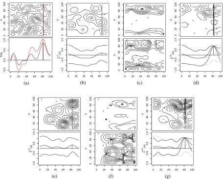
functionθ(x,a)is shown in Figure 1 (a) top. The first input parameter distribution is uniformP[x] =1/100,

thus the sampling procedure must sample across all inputs to learn about the best alternative. The second

distribution is a triangular distribution P[x] =x_10,2₀₀₀ such that the mode input is x=100 and the mean

input is x=66.67 and the sampling procedure must prioritize high P[x]. Given these input parameter

distributions, the true F(a)is calculated via numerical integration and shown in Figure 1 (a) bottom.

At the start of sampling 10 samples are allocated by the random sampling methods described below,

the Gaussain process prediction of θ(x,a) and ˆF10(a) after the initial allocation are shown in Figures 1

(b) and (e) for the uniform and triangular distribution cases respectively. Then the sequential methods are

used to allocate a following 90 samples reaching a full budget of 100, Figures 1 (d) and (g) showθ(x,a)

and ˆF100 after 100 samples have been allocated according to EGO. Then, based on the learned Gaussian

−1 −1 −1 −1 −1 −0.5 −0.5 −0.5 −0.5 −0.5 −0.5 0 0 0 0 0 0.5 0.5 0.5 0.5 1 1 1 1 1 1 1 1.5 1.5 1.5 1.5 2 0 20 40 60 80 100 X −0.6 −0.6 −0.4

−0.4 −0.4

−0.2

−0.2

0

0

0.2 0.2

0.2

0.4

0.4 0.6

0 20 40 60 80 100 ● ● ● ● ● ● ● ● ● ● X 0.2 0.2 0.2 0.4 0.4 0.4 0.6 0.6 0.6 0.8 0.8 0.8 0.8 1 1

1.2 1.4

0 20 40 60 80 100 X ● ● ● ● ● ● ● ● ● ● ● −0.5 −0.5

−0.5 −0.5

0 0 0 0.5 0.5 0.5 0.5

1 1

1.5 1.5 2 0 20 40 60 80 100 ● ● ● ● ● ● ● ● ● ● ● ● ● ● ● ● ● ● ● ● ● ● ● ● ● ● ● ● ● ● ● ● ● ● ● ● ● ● ● ● ● ● ● ● ● ● ● ● ● ● ● ● ● ● ● ● ● ● ● ● ● ● ● ● ● ● ● ● ● ● ● ● ● ● ● ● ● ● ● ● ● ● ● ● ● ● ● ● ● ● ● ● ● ● ● ● ● ● ● ● X

0 20 40 60 80 100

−0.5 0.0 0.5 1.0 F(a) (a)

0 20 40 60 80 100

−1.5 −0.5 0.5 1.5 F ^ 10 ( a ) (b) 0.1 0.1 0.1 0.1 0.2 0.2 0.2 0.2 0.3 0.3 0.3 0.3 0.4 0.4 0.4 0.5 0.5 0.5 0.6 0.6 0.6 0.6 0.7 0.7

0 20 40 60 80 100

0 20 40 60 80 100 X ● ● ● ● ● ● ● ● ● ● ● (c)

0 20 40 60 80 100

−1.5 −0.5 0.5 1.5 F ^ 100 ( a ) (d) −0.2 −0.2 −0.1 −0.1 0 0 0.1 0.1 0.2 0.2 0.2 0.2 0.2

0.3 0.3 0.3 0.3 0.3 0.4 0.4 0.4 0.5 0.5 0.7 0 20 40 60 80 100 ● ● ● ● ● ● ● ● ● ● X 0 0.5 0.5 0.5 1 1 1 1 1.5 0 20 40 60 80 100 X ● ● ● ● ● ● ● ● ● ● ● −0.2 −0.2 −0.2 0

0 0

0.2 0.2 0.2 0.2 0.2 0.2 0.2 0.4 0.4 0.4 0.4 0.4 0.6 0.6 0.6 0.8 0.8 1 1.2 1.2 1.4 1.4 1.6 0 20 40 60 80 100 ● ● ● ● ● ● ● ● ● ● ● ● ● ● ● ● ● ● ● ● ● ● ● ● ● ● ● ● ● ● ● ● ● ● ● ● ● ● ● ● ● ● ● ● ● ● ● ● ● ● ● ● ● ● ● ● ● ● ● ● ● ● ● ● ● ● ● ● ● ● ● ● ● ● ● ● ● ● ● ● ● ● ● ● ● ● ● ● ● ● ● ● ● ● ● ● ● ● ● ● X

0 20 40 60 80 100

−1.5 −0.5 0.5 1.5 F ^ 10 ( a ) (e) 0.1 0.1 0.1 0.1 0.1 0.1 0.1 0.2 0.2 0.2 0.3 0.3 0.3 0.3 0.3 0.4 0.4 0.4 0.4 0.4 0.4 0.5 0.5

0.5 0.5

0.6 0.6 0.6 0.6 0.6 0.6

0.7 0.7

0 20 40 60 80 100

0 20 40 60 80 100 X ● ● ● ● ● ● ● ● ● ● ● (f)

0 20 40 60 80 100

−1.5 −0.5 0.5 1.5 F ^ 100 ( a ) (g)

Figure 1: In all plotsAis on the horizontal axis, small points represent function evaluations. (a)θ(x,a)and

F(a)measured using the uniform test inputs (black) and triangular test inputs (red). µ10(x,a)and ˆF10(a)

with upper and lower confidence bounds after 10 samples are shown for uniform inputs (b) and triangular

inputs (e). (c)and (f) top EGO(x,a), bottomKG(x,a) after the initial 10 samples with uniform inputs (c)

and triangular inputs (f), large points show the peaks. (d) and (g) µ100(x,a) and ˆF100(a) (with ˆF10(a)in

grey) after 100 samples allocated by EGO, (d) uniform and (g) triangular.

recommended to the user

a∗=argmax

a0 ˆ

FN(a0) =argmax

a0 1

1000_x

∑

i∈XR

µN(xi,a0)

where ˆFN(a)is optimised by evaluating for all integer valuesa∈0,1, ...,100 and the highest value is used

as a seed for sequential parabolic interpolation to find the optimal a∗ to high accuracy.

The quality of the sampling procedure is determined by the opportunity cost, the difference in true performance between the design with the highest predicted value and the true best design, which is measured

over a separate random sample of 1000 inputs Xtest that have not been used in the algorithm. The true

value of a given alternative is calculated by

F(a) = 1

1000_x

∑

i∈Xtest

●

●

20 40 60 80 100

5

10

20

50

100

200

Budget N

OC

UNI OC

(a)

20 40 60 80 100

10

20

50

100

200

Budget N

OC

WEDGE OC TRIANGULAR OC

(b)

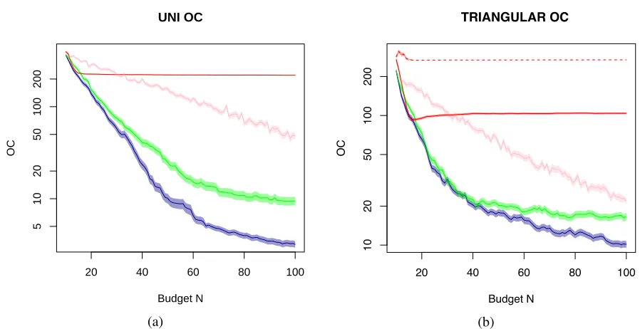
Figure 2: (a) the opportunity cost when the input distribution is uniform, (b) when the input distribution is triangular. EGO on the mean input (red, solid) and mode input (red, dashed) perform worst, followed by Random Sampling (pink) which is significantly worse than EGO (green) and KG (blue).

Therefore the opportunity cost is given by

Opportunity Cost = max

a0

F(a0)−F(a∗). (25)

Code is available online for all experiments and benchmarks athttp://www2.warwick.ac.uk/fac/cross fac/

complexity/people/students/dtc/students2013/pearce/.

5.1 Benchmark Methods

• Random SamplingGiven a budgetN, samples are randomly distributed over the joint input-design space by Latin Hyper Cube (in the uniform input case) or by sampling from the input distribution

and latin hypercube in theAspace. We consider this the simplest uninformed brute-force approach.

• EGO on the mean and mode input We apply a single parameter EGO to the mean input and to

the mode input. This represents a typical approach used in practice, where the input uncertainty is simply reduced to using the most likely or most typical input parameter value. Technically this is equivalent to using the EGO algorithm described above with only one constant sample in the

Monte-Carlo integral. In the uniform case we only use the mean inputx=50, and in the triangular

case we use the meanx=66.67 and the mode x=100. At the end of sampling the bestaon the

single input alone is recommended while opportunity cost is measured over all test inputs.

5.2 Results

ˆ

Fn(a) provides a point estimate of the true performance, ∑θ(xi,a), averaged over a given set of inputs,

XMC, the posterior variance of the estimate is given by

1

N2

X xi∈

∑

∑

and is plotted in Figure 1 as confidence bounds. In Figures 1 (d) and (g) it can be seen that samples are

focussed around the true optimala and the error in ˆF100(a) is much lower around the optimala.

In Figure 2, in both cases applying EGO to the mean input and the mode input results in the opportunity cost not decreasing to zero and the algorithm converges to the wrong design, so reducing input uncertainty to just a typical input parameter value can clearly lead to inferior solutions. In this example, the EGO focusing on the mode input even converges to a solution that is worse than the solution obtained after the initial 10 samples of the methods that take input uncertainty into account. Of the methods that account for input uncertainty, KG works best, followed by EGO and then the simply random sampling.

6 CONCLUSION

When building a simulation model, the user usually faces the challenge to define proper input distributions. Input uncertainty arises when one is not completely certain what distributions and/or parameters to use. In this paper, we proposed two simulation optimization methods based on EGO and KG ideas that are capable to take into account input uncertainty, and identify the design that has the best expected performance over the assumed known distribution of input distribution parameters.

Numerical experiments demonstrated that the new algorithms indeed sample the search space very efficiently, and are much more efficient than random sampling. The approach to simply use EGO on a typical input distribution parameter such as the mode or the mean of the assumed distribution clearly performed worse, which demonstrates the importance of properly accounting for input uncertainty.

There are various avenues for future work. While we assumed in this paper that the design space and the input distribution parameter space can each be described by a single continuous parameter, the proposed methods should also be tested in higher dimensions and with discrete parameters. It would be interesting

to examine the impact of parameter Nx. Finally, one could consider worst case performance rather than

expected performance.

REFERENCES

Branke, J., S. E. Chick, and C. Schmidt. 2007. “Selecting a selection procedure”.Management Science53

(12): 1916–1932.

Branke, J., S. Meisel, and C. Schmidt. 2008. “Simulated annealing in the presence of noise”.Journal of

Heuristics14 (6): 627–654.

Chen, C.-H., S. E. Chick, L. H. Lee, and N. A. Pujowidianto. 2015. “Ranking and Selection: Efficient

Simulation Budget Allocation”. InHandbook of Simulation Optimization, 45–80. Springer.

Fan, W. L., J. Hong, and X. Zhang. 2013. “Robust selection of the best”. InProceedings of the 2013 Winter

Simulation Conference, edited by R. Pasupathy, S.-H. Kim, A. Tolk, R. Hill, and M. E. Kuhl, 868–876. Piscataway, New Jersey: Institute of Electrical and Electronics Engineers, Inc.

Frazier, P., W. Powell, and S. Dayanik. 2009. “The knowledge-gradient policy for correlated normal beliefs”.

INFORMS journal on Computing21 (4): 599–613.

Gao, S., H. Xiao, E. Zhou, and W. Chen. 2016. “Optimal computing budget allocation with input uncertainty”. In Proceedings of the 2016 Winter Simulation Conference, edited by T. M. K. Roeder, P. I. Frazier, R. Szechtman, E. Zhou, T. Huschka, and S. E. Chick, 839–846. Piscataway, New Jersey: Institute of Electrical and Electronics Engineers, Inc.

Huang, D., T. Allen, W. Notz, and R. Miller. 2006. “Sequential kriging optimization using multiple-fidelity

evaluations”.Structural and Multidisciplinary Optimization 32 (5): 369–382.

Jones, D. R., M. Schonlau, and W. J. Welch. 1998. “Efficient global optimization of expensive black-box

functions”.Journal of Global optimization 13 (4): 455–492.

Lam, H. 2016. “Advanced tutorial: Input uncertainty and robust analysis in stochastic simulation”. In

R. Szechtman, E. Zhou, T. Huschka, and S. E. Chick, 178–192. Piscataway, New Jersey: Institute of Electrical and Electronics Engineers, Inc.

Scott, W., P. Frazier, and W. Powell. 2011. “The Correlated Knowledge Gradient for Simulation Optimization

of Continuous Parameters using Gaussian Process Regression”.SIAM Journal on Optimization21 (3):

996–1026.

Song, E., B. L. Nelson, and L. J. Hong. 2015. “Input uncertainty and indifference-zone ranking & selection”. InProceedings of the 2015 Winter Simulation Conference, edited by L. Yilmaz, W. K. V. Chan, I. Moon, T. M. K. Roeder, C. Macal, and M. D. Rossetti, 414–424. Piscataway, New Jersey: Institute of Electrical and Electronics Engineers, Inc.

Zhang, X., and L. Ding. 2016. “Sequential sampling for Bayesian robust ranking and selection”. In

Proceedings of the 2016 Winter Simulation Conference, edited by T. M. K. Roeder, P. I. Frazier, R. Szechtman, E. Zhou, T. Huschka, and S. E. Chick. Piscataway, New Jersey: Institute of Electrical and Electronics Engineers, Inc.

Zhou, E., and W. Xie. 2015. “Simulation Optimization when facing input uncertainty”. In Proceedings

of the 2015 Winter Simulation Conference, edited by L. Yilmaz, W. K. V. Chan, I. Moon, T. M. K. Roeder, C. Macal, and M. D. Rossetti, 3714–3724. Piscataway, New Jersey: Institute of Electrical and Electronics Engineers, Inc.

AUTHOR BIOGRAPHIES

MICHAEL PEARCEis currently a PhD student at the University of Warwick’s Complexity Science Centre.

He graduated from the University of Bristol in 2009 with MSci. in Mathematics and in 2015 with an MSc

in Complexity Science from the University of Warwick. His e-mail address [email protected].

JUERGEN BRANKE is Professor of Operational Research and Systems of Warwick Business School,

University of Warwick, UK. He is Associate Editor for IEEE Transaction on Evolutionary Computation, Associate Editor for the Evolutionary Computation Journal, and Area Editor for the Journal of Heuristics. His research interests include metaheuristics, multiobjective optimisation and decision making, optimisation in the presence of uncertainty, and simulation-based optimisation, and he has published over 160