A Fixed Point Method for Convex Systems
Morteza Kimiaei1, Farzad Rahpeymaii2
1Department of Mathematics, Razi University, Kermanshah, Iran 2Department of Mathematics, Payame Noor University, Tehran, Iran
Email: [email protected], [email protected] Received June 26, 2012; revised September 27, 2012; accepted October 6, 2012
ABSTRACT
We present a new fixed point technique to solve a system of convex equations in several variables. Our approach is based on two powerful algorithmic ideas: operator-splitting and steepest descent direction. The quadratic convergence of the proposed approach is established under some reasonable conditions. Preliminary numerical results are also reported.
Keywords: Convex Equations; Least Squares; 1-Regularization Problems; Fixed Point; Quadratically Convergence
1. Introduction
System of convex equations is a class of problems that is conceptually close to both constrained and unconstrained optimization and often arise in the applied areas of mathe- matics, physics, biology, engineering, geophysics, chemistry, and industry. Consider the following system of convex equations
0, nF x xR
m
(1)
in which F R: nR is a convex continuously differ-
entiable function. It is noticed that if F x
Axm n
b the system (1) is a linear system of equations and there are a lot of approaches to solve this problem. One of the most interesting methods for solving linear system is fixed point methods that have been comprehensively studied by many authors. For example, shrinkage, subspace optimization and continuation [1], fixed-Point continuation method [2], nonlinear wavelet image processing [3], EM method [4], iterative thresholding method [5] and fast iterative thresholding [6]. The system (1) is called an overdetermined system whenever and under-de- termined for nm. If m n , we obtain a square system of convex equations. Most of the time, we wish to find a proper x R n such that (1) holds as closely as
possible. This means that our objective is to reduce
2F x as much as and, if possible, reduce it to zero. Hence the system of convex Equations (1) can be written as an unconstrained optimization problem
minf x s.t x R n (2)
in which
22
1 .
2
f x F x (3)
It is obvious that
T
,g x f x J x F x
where J x
is the Jacobin matrix of F x
. In this work, we consider a -regularized least squares problem for system (1): 1
1
min x x f x (4)
in which 0
, , ,F Fmis a parameter. We note that if 1 2
and any iT
F F F is convex, then F is
convex. On the other hand, convexity of 22 implies that f is convex. Therefore, φ is a convex function.
.
As an example, Hale, Yin, and Zhang in [2] presented a fixed-point continuation method for 1-regularized minimization that based on operator-splitting and con tinuation:
1 shrink ,
k k
x h x (5)
in where
and mappings shrink, :h RR are
defined as :
,h I g (6)
shrink sgn max | | ,0 .
(7)The operator in the right hand side of relation (7) denote the component-wise product of sgn
and
max | | ,0 . Because of the parameter τ is constant, the number of iterations and computational costs increase and so it is not suitable. To overcome the mentioned disadvantage, we create innovation in the parameter τ
kT k kT
k k k k
g g
J g J g
(8)
The analysis of the new approach shows that it inherits both stability of fixed point methods and low com- putational cost of steepest descent methods. We also in- vestigate the global convergence to first-order stationary points of the proposed method and provide the quadratic convergence rate. To show the efficiency of the proposed method in practice, some numerical results are also reported.
The rest of this paper is organized as follows: In Section 2, we describe the motivation behind the pro- posed algorithm in the paper together with the algo- rithm’s structure. In Section 3, we prove that the proposed algorithm is globally convergent. Preliminarily numerical results are reported in Section 4. Finally, some conclusions are expressed in Section 5.
2. The New Algorithm: Motivation and
Structure
In this section, we first introduce a fixed point algorithm for small-scale convex systems of equations. Then, given some properties of the algorithm and investigate its global convergence as well as the quadratic convergence rate. The objective function in (4) is a sum of two convex functions. By convex analysis, minimizing a convex function
x is equivalent to finding a zero of the subdifferential
x . Let X* be the set of optimal solutions of (4). It is well-known that an optimality condition for (4) is
* * 0 sgn * *
,x X x g x
or equivalently,
*
* * * *
*
1 0
1,1 0
1 0
i i i
x
x X g x x
x
(9)
where 0 denotes the zero vector in Rn and *
i
x is i-th component of x*. It follows readily from (9) that 0 is an optimal solution of (4) if and only if g
0 1, or in other words,
* 1
0
0
X
g
Therefore, it is easy to check whether 0 is a solution of (4) (see [2]).
One of the simplest methods for solving (4) generates a sequence
that based on steepest de-0
k k k
k
x g
scent direction. Here,
kT k k
T
k k k k
g g
J g J g
and gk J Fk k. Note that if the system (1) be a linear
system of equations, then g 2A AT and
max
2
0, T
A A
k
. Here, the system (1) is a convex
system of equations, then gk J JkT and for the
purpose of our analysis, we will always choose
max
1
0 k
kT k
J J
. Using these information, we
present a proximal regularization of the linearized function f at xk for problem (4) (see [7]), and written it
equivalently as
12
1 2
arg min
1 1
. 2
k k k kT k
x
k
k k
fx f x g x x
x x x
(10)
After ignoring constant terms, (10) can be rewritten as
2 1
1 2
2
1
1 1
arg min 2
arg min | | .
2
k k k k k
k
k k
n
i k k k
x k i i
i
x x x g x
x x g x
(11)
Notice that the function in the problem (11) is minimized if and only if each functions
2 ,2
k
k k k
i k i i i i1, 2, , n
q x x x g x
is minimized. If we take
k k
k
, then we can simply
obtain the minimizer of q xi
as follows:
* 0
k k k k
k k k k
i i
k k k k
i i
k k k k
k k k
i
i
x g
x g
x x
x g x g k
g
* Therefore, k 1 i
i
x x and the solution of (4) is
obtained. Now, based on above arguments, a new fixed point algorithm can be outlined as follows:
Algorithm 1: Fixed point algorithm (FP)
Input: Choose an initial point x0Rn and constants
0
, 00 1,
1,10 . Begin0 1
; k0l
While
k 2 max
Step 1: {Parameter shrinkage calculation}
andk k
;
k k
k
Step 2: {Operation shrinkage calculation}
1 shrink ;
k k
x h x
Step 3: {Parameters update} Calculate k as (8);
Generate k1k;
Increment k by one and go to Step 1; End While {End loop}
End
3. Convergence Analysis
In this section, we will give the convergence analysis of the proposed algorithm given in Section 2. In the convergence analysis, we need the following assumption:
(H1) Problem (4) has an optimal solution set X* , and there exists a set
*
*2
: δ ,
x x x X
for some x*X* and , such that f is twice continuously differentiable on Ω and
δ0
max
ˆ T max T ,
x
J x J x J x J x
for all x . Using the mean-value theorem, we hav
1
0
, , ,
T
T
g x g y J y t x y J y t x y
J x y J x y x y
Tfor any x y, .
(H2) There exists a constant M 0 such that
k ,
0 .J x M k N
Lemma 3.1. By the definition of i and j satisfy- ing (8), we have
i j i
x x j
for any x xi, j .
Proof. Suppose that xixj then gigj and
iT i jT j
J J J J . So by (8), we conclude that igi jgj.
Now suppose that ij. Then, we show that xixj.
By contradiction, we assume that xi xj . Then
i j
g g and J JiT iJjT j
i i J . j j
Therefore we have g g that is a contradiction. In the following lemma, we show that the new choice of k satisfying in the lemma 4.1 and corollary 4.1 of
[2] when
max
1 0, k
kT k
J J
.
Lemma 3.2. Under assumption (H1), the choice of i and j result in h
I
g
,
i j
x x
is nonexpansive over Ω, i.e. for any
2 2.i j i j
h x h x x x (12)
Moreover, gigj whenever equality holds in (12).
Proof. Let J J x x
i j and dxixj. Now, we have two cases:1) If j i, then
i j i j i i jh x h x x x g gj (13)
d d
d.
i i j i T
i T
g g J
I J J
J
Hence,
i j 2
i T
d2 h x h x I J J2 2
i T i j
I J J x x
2ˆ
max 1 i J JT ,1 xi xj
2ˆ ˆ
max ,1 .
ˆ
iT i T
i j
iT i
J J J J
x x J J
Let pJd . By the lemma 3.1, we have
dxixj 0 if and only if igijgj 0.
Then
2 d2 d
2 d2i j i i j j
h x h x g g
2dT igi jgj igi jgj T igi jgj 0
2d
T
j j i i j j i i
T i i j j
g g g g
g g
if igijgj 0,
by the equation (13), we obtain
1 2 1 2 ,
d d
T
i T i T i T T
i T T T
J J J J p J Jp
J J p p
which contradicts to ˆ
T T
T T
p J Jp J J
p p .
Hence p0 so that
i j T 0.g x g x J p
2) If ij, then
j i j i j j i
d d
d.
j j i j T
j T
g g J J
I J J
Hence,
j i 2
j T
d h x h x I J J2
2 2
j T j i
I J J x x
2ˆ
max 1 j J JT ,1 xj xi
2ˆ ˆ
max ˆ ,1 .
jT j T
j i
jT j
J J J J
x x J J
Let pJd. By the lemma 3.1, we have
dxixj0 if and only if jgjigi 0.
Then
2 d 2 d
d 2j i j j i i
h x h x g g 2
2dT jgj igi jgj igi T jgj igi 0
2d
T
i i j j i i j j
T j j i i
g g g g
g g
if jgjigi 0, by the Equation (14), we obtain
1 2 1 2 ,
d d
T
j T j T j T T
j T T T
J J J J p J Jp
J J p p
which contradicts to ˆ
T T
T T
p J Jp J J
p p . Hence p0 so that
j i T 0,g x g x J p
which completes the proof.
Corollary 3.3. (Constant optimal gradient). From (H1) assumption, for any , there is a vector
such that
* * x X
* *g x
*Rn
.
Let X* be the solution set of (4), x*X*, and * be the vector specified in corollary 3.2. Then, we define
: * 1 ,
: *
i i
L i E i 1 ,
1 * :
i i
,
where
. We will show that the sequence gener-
ated by (5) is finite convergence for components in L and is quadratic convergence for components in E.
It is obvious from the optimality condition (9) that
L E {1, 2, , n}, and for any x*X*, we have
* *
supp x i x: i0 E,
* 0, .
i
x i L
Hale, Yin, Zhang in [2] establishes the finite con- vergence properties of
xk stated in the following oftheorem. The proof of the theorem 3.4 and 3.5 is similar to the theorem 4.1 and 4.2 in [2].
Theorem 3.4. Under assumption (H1), the sequence
xk is generated by the fixed point iteration (5) appliedto problem (4) from any starting point x0 converges to some x*X* . In addition, for all but finitely many iterations, we have
* 0
k
i i ,
x x i L (15)
*
*sgn k sgn ,
i i i
h x h x g i L (16)
where the numbers of iterations not satisfying (15) and (16) do not exceed x0x*2 2 and x0x*2 2, respectively.
Theorem 3.5. (The quadratic case). Let f be a convex quadratic function that is bounded below, J JkT k be its
Hessian, and k satisfy
max 1
0, ,
k
kT k
J J
then the sequence
xk is generated by the fixed pointiteration (5) applied to problem (4) from any starting point x0 converges to some . In addition, for all but finitely many iterations, we have (15) - (16) hold for all but finitely many iterations.
* * x X
Lemma 3.6. Suppose assumptions (H1) and (H2) holds. Then, we have
2
limk Fk 0.
Proof. From (9), we can obtain 1,
k k g
then, by (H2) and the above inequality, we have
2
1
1 .
k k k k
k
M F F F
M
For sufficiently large k, we conclude that
2 limk Fk 0.
Now, consider the sequence
xk generated by the FPalgorithm. According to the fixed point iterations (5), it converge to some point x*X* . We will show that the convergence is quadratic. In order to do, the following additional assumption is required:
(H3) The following condition
1
,k k k k
holds, in where Gk J x x
k, k1
TJ x xk, k1
k . Suppose that k is enough large so and
that
, for all . Also, suppose thatT
k k
G J x J x
* 0
k
i i
x x i L
, , ,
EE i j i j E
C C
denote the square sub-matrix of the matrix C cor- responding to the index set E. Firstly we suppose that
*
, then the mean-value theorem yields
k * k * k i * *E E E E E E E
h x h x x x g gE (18)
* * *
*
k k k k k k k
E E E E E E E E EE E E
k k k
E EE E E
*
x x g g x x G x x
I G x x
Since xk 1
shrink h x
k and shrink .
is
non-expansive [2], using H2, (17), and (18), we have that
1 * 1 * *
2 2 2
k k k
E E E E E E
x x x x h x h x
* kT k *
k k k E k k
E EE E E kT k k EE E E
E EE E
g g
I G x x I G x x
g G g
*
kT k k kT k k
k
E EE E EE
E E
kT k k
E EE E
g G g g G g
x x
g G g
*kT k k k
E EE EE k
E E
kT k k
E EE E
g G G g
x x
g G g
2 * *
2 2
2 2 2
*
* 2
2 *
2 .
k k k k
EE EE EE EE
k k
E E E
k E
k
k
k
G G G G k
g x x x x
M M g
O x x
x x
M
O x x
M
Secondly, we suppose that k *. Similar first case, we conclude that
2
1 * *
k k
x x O x x .
Theorem 3.7. Suppose that (H1)-(H3) holds and let
xk is the sequence generated by the FP algorithmstarting x0 . For sufficiently large k, the sequence
xk is converges to some point in X* quad- ratically.4. Preliminary Numerical Experiments:
This section reports some numerical results and com- parisons regarding the implementations of the new pro- posed idea of the present study with some other algo- rithms for small-scale problems. All codes are written inMATLAB 9 programming environment with double precision format by a same subroutine. In the experi- ments, the presented algorithms are stopped whenever
k 10 .5F x
Test problems are as follows: 1) Tridiagonal system linear is
,F x Ax
in where A is a n n tridiagonal matrix given by
tridiag 1,8, 1 ,
A
and
:,
:, , : 1, , :,A i
A i i i
A i
n
2) Five diagonal system linear is
,F x Ax
in where A is a n n five matrix given by
tridiag 1, 1,8, 1,1
A
and
:,
:, , : 1, , :,A i
A i i i
A i
n
3) Logarithmic function [8]
ln
1
i, 1, , ,i i
x
F x x i
n
n
initial point: x0
1, ,1
.4) Strictly convex function 1 [8] f x
that is the gra-dient of
1ei n
x i i
h x x
exi 1, 1, ,i ,
F x i n
initial point: x0 1 2, ,n
n n n
.
5) Strictly convex function 2 [8] f x
that is the gra-dient of
1
e 10
i n
x i i
i
h x x
e 1 ,
1, , 10i
x i
i
F x i n
initial point: x0
1, ,1
.6) Strictly convex function 3 [8] f x
that is the gra-dient of
1e 10
i
n
x i
i
x i
h x
i
e 1 , 1, ,10
i x i
i
,
F x i
i
initial point: x0
1, ,1
. 7) Linear function-full rank [8]
1
2 n , 1, ,
i i j
j
F x x x i
n
ninitial point: x0
100, ,100
. 8) Penalty function [8]
105
1 ,
1, , 1,i i
F x x i n
21
1 1
,
4 4
n j n
j
F x x
n
initial point: 0 1, ,1
3 3
x
. 9) Sum square function [9]
, 1, ,i i ,
F x ix i n
initial point: x0
1, ,1
.10) Trigonometric exponential function [10]
1 1 exp cos 1 2 ,
F x x h x x
exp cos
1 1
,i i i i i
F x x h x x x
1
2, , 1, n n exp cos n n
i n F x x h x x ,
where h h n 1.
initial point: x0
1.5, ,1.5
.In this section, we compare the numerical results obtained by running Algorithms following:
1) FP1
k 1
2) FP2
kT k k
k
k k k k
g g J g J g
3) DS (steepest descent direction,
.kT k k
k k k T k k
g g
d g
J g J g
in where the Jacobian matrix Jk is exact. In running the
algorithm FP1 and FP2 takes advantages of the parame - ters0 1,0 1 g0 ,
0 0.005 g0 ,
10 and
max . The dimensions of problems are selected from 2 to 100. The results for small-scale problems are summarized in Table 1.
1000
k
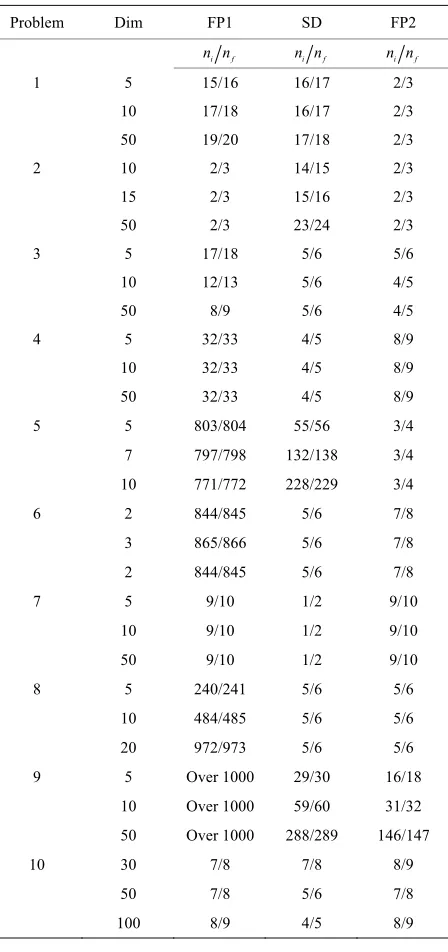
In Table 1, ni and nfrespectively indicate the total
number of iterates and the total number of function eva- luations. Table 1 indicates the total number of iterations and function evaluations for some small scale problems with dimensions 2 to 100. Evidentally, one can see that FP2 performs better than the other presented algorithms in the sense of both the total number of iterations and the total number of function evaluations. From Table 1, we ob-
serve that the proposed algorithm is the best one on the all of test problems. We can deduce that our new algo- rithm is more efficient and robust than the other con- sidered algorithms for solving small scale system of convex equations problems. In more details, the results of Table 1 in Figure 1 are interpreted thanks to the Dolan and More’s performance profile in [11].
[image:6.595.51.284.71.577.2]In the procedure of Dolan and More, the profile of each code is measured considering the ratio of its com- putational outcome versus the best numerical outcome of all codes. This profile offers a tool for comparing the performance of iterative processes in statistical structure. In particular, let Sis set of all algorithms and P is a set of
Table 1. Numerical results for small scale problems.
Problem Dim FP1 SD FP2
i f
n n n ni f n ni f
1 5 15/16 16/17 2/3
10 17/18 16/17 2/3
50 19/20 17/18 2/3
2 10 2/3 14/15 2/3
15 2/3 15/16 2/3
50 2/3 23/24 2/3
3 5 17/18 5/6 5/6
10 12/13 5/6 4/5
50 8/9 5/6 4/5
4 5 32/33 4/5 8/9
10 32/33 4/5 8/9
50 32/33 4/5 8/9
5 5 803/804 55/56 3/4
7 797/798 132/138 3/4
10 771/772 228/229 3/4
6 2 844/845 5/6 7/8
3 865/866 5/6 7/8
2 844/845 5/6 7/8
7 5 9/10 1/2 9/10
10 9/10 1/2 9/10
50 9/10 1/2 9/10
8 5 240/241 5/6 5/6
10 484/485 5/6 5/6
20 972/973 5/6 5/6
9 5 Over 1000 29/30 16/18
10 Over 1000 59/60 31/32
50 Over 1000 288/289 146/147
10 30 7/8 7/8 8/9
50 7/8 5/6 7/8
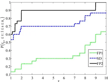
[image:6.595.313.537.266.742.2]Figure 1. Performance profile for the number of iterates.
test problems, with ns solvers and np problems. For
each problem p and solver s and p s, is the computation result regarding to the performance index. Then, the following performance ratio is defined
t
,
,
,
min :
p s p s
p s
t r
t s S
(19)
If algorithm is not convergent for a problem p, the procedure sets p s, fail, where fail should be strictly larger than any performance ratio (19). For any factor
s
r r r
, the overall performance of algorithm is given by
s
,
1
size : .
s p
p
p P r
n s
In fact s
is the probability of algorithm s Sthat a performance ratio rp s, is within a factor R of the best possible ratio. The function s
is thedistribution function for the performance ratio. Especially, gives the probability that algorithm s wins over all other algorithms, and s
1
,p s
r s
lim
gives the probability of that algorithm s solve a problem. Therefore, this performance profile can be considered as a measure of the efficiency and the robustness among the algorithms. In Figure 1, the x-axis shows the number while the y-axis inhibits
p s, :1 s
.P r s n
From Figure 1, it is clear that FP2 had the most wins compared with the other algorithm while it solved about 60% of the test problems with the greatest efficiency. If one concentrates on the ability of completing a run successfully, it can be seen that FP2 is the best algorithm among the considered algorithms because it reaches faster than the other.
5. Conclusion
In this paper, we have presented a new algorithm for
small-scale systems of convex equations that blending steepest descent direction and fixed point ideas. Preliminary numerical effort on the set of small-scale convex systems of equations indicates that significant profits in both the total number of iterations and the total number of function evaluations can be achieved.
REFERENCES
[1] Z. Wen, W. Yin, D. Goldfarb and Y. Zhang, “A Fast Algorithm for Sparse Reconstruction Based on Sharin- kage,” Optimization, and Continuation, CAAM Technical Report TR09-01, 2009.
[2] E. T. Hale, W. Yin and Y. Zhang, “A Fixed-Point Continuation Method for 1-Regularized Minimization with Applications to Compressed Sensing,” CAAM Tech- nical Report TR07-07, 7 July 2007.
[3] A. Chambolle, R. A. De Vore, N. Y. Lee and B. J. Lucier, “Nonlinear Wavelet Image Processing: Variational Pro- blems, Compression, and Noise Removal through Wave- let Shrinkage,” IEEE Transactions on Image Pro- cessing, Vol. 7, No. 3, 1998, pp. 319-335.
doi:10.1109/83.661182
[4] M. A. T. Figueiredo and R. D. Nowa, “An EM Algorithm for Wavelet-Based Image Restoration,” IEEE Trans-
actions on Image Processing, Vol. 12, No. 8, 2003, pp.
906-916. doi:10.1109/TIP.2003.814255
[5] I. Daubechies, M. Defrise and C. D. Mol, “An Iterative Thresholding Algorithm for Linear Inverse Problems with a Sparsity Constraint,” Communications on Pure and
Applied Mathematics, Vol. 57, No. 11, 2004, pp. 1413-
1457. doi:10.1002/cpa.20042
[6] C. Vonesch and M. Unser, “Fast Iterative Thresholding N. Algorithm for Wavelet-Regularized Deconvolution,” Pro-
ceedings of the SPIE Optics and Photonics 2007 Con-
ference on Mathematical Methods: Wavelet XII, Vol.
6701, San Diego, 26-29 August 2007, p. 15.
[7] B. Martinet, “Régularisation d’Inéquations Variation Nelles par Approximations Successives,” Recherche Oper-
ationnelle, Vol. 4, No. 3, 1970, pp. 154-158
[8] G. L. Yuan, Z. X. Wei and S. Lu, “Limited Memory BFGS Method with Backtracking for Symmetric Non- linear Equations,” Mathematical and Computer Modelling, Vol. 54, No. 1-2, 2011, pp. 367-377.
doi:10.1016/j.mcm.2011.02.021
[9] M. Moga and C. Smutnicki, “Test Functions for Op- timization Need,” 2005.
www.zsd.itc.pwr.pc/file/docs/function.pdf.
[10] L. Lukšan and J. Vlček, “Sparse and Partially Separable Test Problems for Unconstrained and Equality Con- strained Optimization,” Technical Report, Vol. 767, 1999. [11] E. D. Dolan and J. J. Moré, “Benchmarking Optimization
Software with Performance Profiles,” Mathematical Pro-