Multi axis numerical control

A thesis submitted for the degree of Master of Engineering

in the

University of Canterbury New Zealand

ACKNOWLEDGEMENTS

I am indebted to my supervisor Dr G R Dunlop for his guidance, encouragement and

help during the course of this research and preparation for this thesis. I am grateful to

Mr N Bolland for his sincere concern and help.

I wish especially to present this to my husband Xiao Xuan, for his strong

encouragement and support, and to all of my family for their significant help.

Finally. my thanks go to all those who assisted me in many ways with their

CONTENTS

ACKNOWLEDGEMENTS I

ABSTRACT IV

PUBLISHED PAPERS V

LIST OF SYMBOLS VI

CHAPTER 1 INTRODUCTION 1

1.1 Robotics 2

1.2 Satellite Tracking - The "Key Hole" Problem 3

1.3 The Stewart Platform 5

CHAPTER 2 NUMERICAL CONTROL OF MULTI-AXIS MACHINERY 13

2.1 Introduction 13

2.2 Single Motor Control Problem 14

2.3 Multiple Motor Control Problem 17

2.4 Accurate Multiple Motor Control 18

CHAPTER 3 DESIGN OF A MULTI-MOTOR CONTROLLER 26

3.1 Introduction 26

3.2 The Computer and Its I/O Channel 27

3.3 The HCTL-lOOO 28

3.3.1 The Operation 28

3.3.2 User Accessible Registers 29

3.3.3 Timing Diagram 30

3.4 Design of the Controller 31

3.4.1 IBM-PC I/O Bus 31

3.4.2 Decoder and Control Logic 31

3.4.2.1 Clock 31

3.4.2.2 Control Signals Decoding 32

3.4.2.3 Data Transfer 33

3.4.2.4 An Example 33

3.4.3 Reset 33

3.4.4 HCTL-1000 34

3.4.5 Buffer 35

3.4.6 Controller Socket 35

3.5 Testing 35

CHAPTER 4 DC MOTOR PWM SERVO DRIVE 51

4.2 DC Motor 52

4.2.1 Operation Principles 52

4.2.2 Classification and Characteristics 53

4.2.2.1 Shunt Motor 54

4.2.2.2 Series Motor 54

4.2.2.3 Compound Motor 55

4.2.2.4 Separately Excited Motor 55

4.2.2.5 Constant Field and Permanent Magnetic DC Motors 55 4.2.2.6 Motor Parameters

4.3 DC Motor PWM SeIVo Drive 4.3.1 Introduction

57 58 58

4.3.2 Three Modes of PWM Drives 59

4.4 Design and Testing 59

4.4.1 Bipolar PWM SeIVo Drive 59

4.4.1.1 Logic Design 59

4.4.1. 2 PWM Drive Design 61

4.4.1.3 Problem and Analysis 62

4.4.2 Limited Unipolar PWM SeIVo Drive 62

4.4.3 Motor Performance 63

4.5 SUITllDary 64

CHAPTER 5 SYSTEM MODELLING AND ANALYSIS 82

5.1 Control Modes 82

5.1.1 Position Control 82

5.1.2 Proportional Velocity Control 83

5.1.3 Integral Velocity Control 84

1.4 Trapezoidal Profile Control 84

5.2 The Electromechanical Model 85

5.2.1 The Motor 85

5.2.2 The Encoder 87

5.2.3 The Control System Modelling 88

5.2.4 Theoretical Response 91

5.3 Experimental Response Analysis 92

5.4 SUITllDary 93

CHAPTER 6 CONCLUSION 105

APPENDIX A SYSTEM PERFORMANCE FOR LARGE STEP INPUTS 107

APPENDIX B ANALYSIS OF FRICTION EFFECTS 109

APPENDIX C PROGRAM LISTING 113

ABSTRACT

This thesis presents the analysis, design and development of a multi-axis machinery

numerical control system. The purpose of this research is to provide a numerical

control method to overcome the multi-axis numerical control problem.

The control system includes an IBM-PC computer as a host processor, a plug in

multi-motor controller board based on commercial numerical multi-motor controller ICs. These

implement a software specified digital control algorithm and output a PWM control

number. Six motors, their driven actuators, and digital incremental feedback encoders

complete the system.

The experimental aspects of the work included the design of the IBM-PC plug in motor

controller board and the motor drive board, computer software for real-time control

and the system testing. For the theoretical aspects of the work, control theory was

used to develop the mathematical model of the system. This aimed at providing a tool

to predict and optimize the system performance, therefore, to fulfill the high

PUBLISHED PAPERS

Dunlop GRand Ma Li: Multi-axis Numerical Control. Proc. IMC Conf., Christchurch, New Zealand, May 1988

Az

El T(f) T_i(f)

J e(t) d T1 T2 0)1 0)6

Tm

JS,

Vm

K

Pm

P

Vs

lAB

y.

dO)

90· -

$,

e,

LIST OF SYMBOLS

(step motor) pull-out torque at a stepping rate f load torque

motor inertia

rotating angle of motor shaft

microprocessor direct control delay value

time taken in the idle path (microprocessor direct control) time taken in the step path (microprocessor direct control) motor velocity in one motor direct control

motor velocity in one motor direct control motor shaft torque

DC motor magnetic flux per pole motor armature current

constant of the motor winding motor back emf voltage motor shaft velocity motor armature resistance motor terminal voltage motor torque constant

motor back emf voltage constant mechanically developed motor power electrical power absorbed in the motor rotor the voltage of the power supply

the current flowing through the motor in PWM servo drive

the current flowing through the motor during the FETs "on" time in PWM servo drive

the current flowing through the motor during the FETs "off' time in PWM servo drive

PWM servo drive input voltage time

K A B

T

Av

Tfr

Vef

a

Kex Kth

PWM%

the motor time constant

the gain number in the register R22H in the HCTL-lOOO the zero number in the register R20H in the HCTL-IOOO the pole number in the register R21H in the HCTL-lOOO sample time

amplitude of a step input torque caused by friction the effective voltage

the effective voltage coefficient

CHAPTER 1

INTRODUCTION

Despite rapid developments in electronics and communications, traditional mechanical

engineering is still an essential part of modern society. In particular, Multi-axis

machinery is an important field which draws on all of these engineering disciplines.

Multi-axis machinery is a type of machinery which has multiple axes or mechanisms,

each of which can execute a required motion to produce a coordinated motion for the

whole machine. The purpose of this type of machine is to do complicated jobs so as to

increase efficiency or reduce costs. Robots, satellite tracking mechanisms and some

machine tools are typical applications of such machines.

The remaining part of this chapter will discuss these applications including their

functions and existing problems, and then give a mechanism as a solution. The second

chapter discusses the numerical control problems associated with ordinary control

means used to drive multi-axis machinery. A satisfactory solution to these problems is

developed.

The later chapters present the design, theoretical analysis and performance of a

multi-axis machine numerical controlleI," developed during this research, i.e. the problems

1.1 ROBOTICS

Since the word "robot" was first introduced in 1917 (McCloy 1986), it has become widely used by many people. Because of the potential shown by robots in substituting people's labour especially in dangerous or boring work, the use of robots is becoming widespread.

According to mechanical arrangement of the manipulators, robots can be divided into two categories: i) The serial or open link manipulators and ii) the parallel or closed link manipulators.

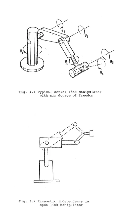
The arrangement of a six degrees of freedom serial link robot is shown in Fig. 1.1. It has six fixed length links and is a traditional type coming from the simulation of the human body, i.e. anthropomorphic. Each link can swing through an arc with respect to the preceding link. Hence, the manipulator has six degrees of freedom and the end effector (or gripper) is positioned within the working volume.

The main advantages of a serial link manipulator are:

-the manipulator has high mobility, Le., has a long reach and a large range of motion since the links are connected one after another;

-it has flexible reaching points, even to corners. The disadvantages are:

-a given set of end actuator coordinates does not have a unique set of joint

coordinates. In other words, the link positions are usually indeterminate (c.f. Fig.

1.2) (Dunlop & Afzulpurkar 1988).

1.2 SATELLITE TRACKING -

THE "KEY HOLE" PROBLEM

Satellites are now the dominant carriers of telecommunications and are playing

important parts in space and the earth resource exploitation. Satellite tracking systems

have been developed since 1963 after the space research started in late fifties. Good

tracking systems must be able to find their satellites quickly and maintain

. communication with them through unexpected orbital changes. For maritime earth

stations, they need also be able to overcome the effect of rolling and pitching of the

ships. The earth station antenna dish diameters may be as large as 30m and can weigh

up to several hundred tons (Afzulpurkar et al 1988). As the frequency used increases,

the beamwidth is reduced, so more than a fraction of a degree of apparent satellite

movement must be tracked (Pratt and Bostian 1986). Hence a good tracking

mechanism is required to ensure the completion of the task On the other hand, they

must be relatively inexpensive.

The present popularly used tracking mechanisms can be generally divided into three

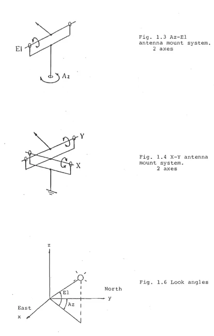
categories: Alt-Azimuth or Az-El mount (c.f. Fig. 1.3), X-Y mount (c.f. Fig. 1.4) and

a combination of these two (c.f. Fig. 1.5 and Miya 1981).

The path followed by any satellite moving around the earth is a decaying ellipse in the

orbital plane. The coordinates to which the antenna must be pointed to communicate

with the satellite are called the "look angles". These are most commonly specified as

geographic north to the intersection of the satellite orbital plane on the horizontal plane

at the earth station. Elevation (900 -

e )

plane to the line of sight of the satellite (c.f. Fig. 1.6).

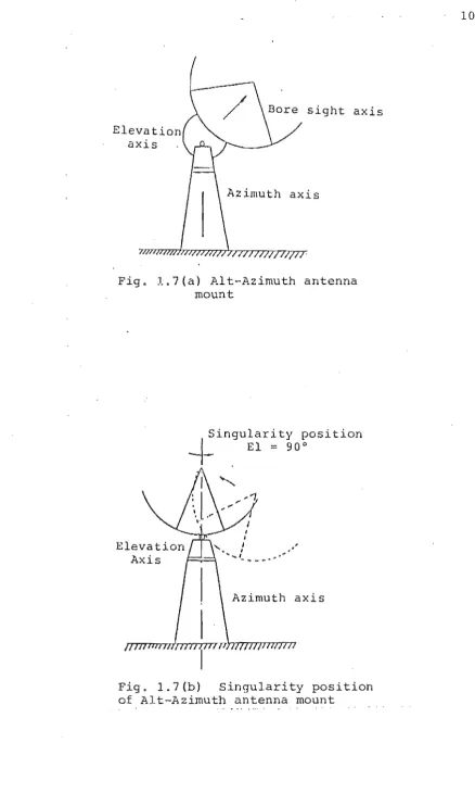
An Az-El type of mounting system has two axes, Az and El. The antenna bore sight

axis will trace a semicircle on a vertical plane about El axis and can sweep a horizontal

circle about Az axis. When a satellite starts approaching to the zenith, Le. the El angle

90° (c.f. Fig. 1.7(a», the antenna dish has to rotate the azimuth angle through 180'"

about the bore sight axis to continue the tracking because of limitations in the

mechanism (c.f. Fig. 1.7(b». Thus the system has a singularity at the zenith. During

the time taken for this 1800 azimuth rotation, the satellite moves out of the beam of a

high gain antenna and the station loses contact with the satellite. This is known as the

"key hole" problem. The problem becomes particularly severe when the tracking

system is mounted on a ship. The rolling and pitching action of a ship causes the

singularity of the Az-El mount to trace out a flattened cone about the zenith. If the

satellite is within this flattened cone region, communication contact can be lost and the tracking ceases. When receiving signals from deep space probes, there is only one·

chance of capturing the data sent by the space craft and such a loss of contact is

unacceptable (Afzulpurkar et alI988).

An X-Y type of mounting system has X and Y axes (c.f. Fig. 1.4). When the antenna

dish tracks a satellite along the horizontal plane and near the axis mountings, the

track in path is occluded by the mountings, so it has to rotate 180· for continuing the

tracking. Thus the "key hole" problem exists along the horizontal axis in an X-Y

mounting system. For overcoming the effect of rolling and pitching of a ship mounted

application, the antenna being able to point below the horizon is needed, so the X-Y

"key hole" problem for deep space work, two ground based X-Y mounted antennas

are mounted perpendicular to each other. Thus the singularity of each antenna is

covered by the other and the signals are received and complementary mutually.

However, the cost of the tracking system is doubled.

The conventional solution to the "key hole" problem is to use a combined mount of

X-Y type and Az-El type (c.f. Fig. 1.5(c) and Miya). A horizontal plane is always

maintained against ship's motions by controlling the X and Y axes of the plane. The

direction to the satellite is produced by controlling the azimuth-elevation axes mounted

on this horizontal plane. Controlling of the X-Y and Az-El axes is independent, but

the cost and complexity of the operation are greatly increased.

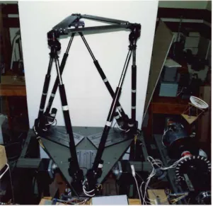
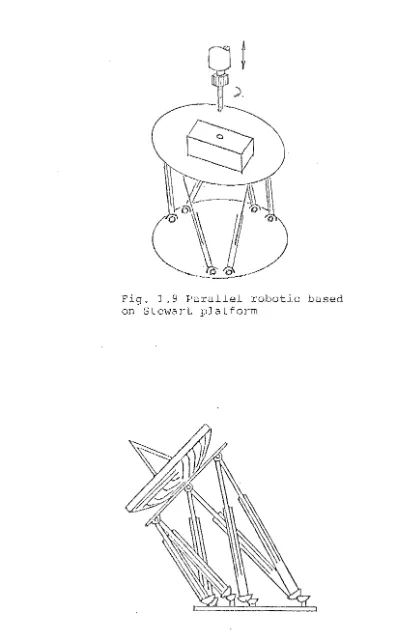
1,3 THE STEWART PLATFORM

The solution to the above problems in robotics and satellite tracking systems is to use a

Stewart platform mechanism (c.f. Fig. 1.8).

The Stewart platform was proposed in 1965 (Stewart) and is widely used for aircraft

simulation and other purposes nowadays. It is a parallel1ink manipulator. It consists

of two bodies connected by six legs. One body is called the base, which is usually

fixed, and the other is called the platform which is movable. Each of the legs is in the

form of a linear actuator. Each actuator has one end joined to the base and the other

end joined to the platfonn. The actuators are prismatic joints and can expand and

contract independently thus positioning the platfonn in space. This arrangement

position and any orientation within a certain work volume. The arrangement of the

structure is symmetric to achieve maximum stiffness.

With this rigid mechanism, the joint deflection problem in serial link robotics is

considerably reduced and high accuracy positioning can be achieved. These properties make it suitable for use in heavy duty environments, such as automotive assembly

applications and the like (c.f. Fig. 1.9).

For the satellite tracking application, an antenna dish is mounted on the platform and a

tracking system with six degrees of freedom is formed. The antenna dish can even

point 30° below the horizon with carefully designed joints (c.f. Afzulpurkar et al

1988). When this mechanism is applied in a ship mounted environment, it is able to

track the satellite rapidly without mechanism singularity limitations, therefore is a

rather simple and reliable mechanism to overcome the "key hole" problem (c.f. Fig.

L 10). The six identical actuators simplify the manufacture.

So far the solution to the problem raised in 1.1 and 1.2 has been clearly given - the

Fig. 1.1 Typical se~iel link manipulator with six degree of freedom

" ' 1 - - - - ' - - (

/'" 0

E\

~Az

z

\

East

x

North y

Fig. 1.3 Az-El

antenna mount system. 2 axes

Fig. 1.4 X-Y antenna

mount system. 2 axes

Cross-E\

~Az

x

(a) Az, El,

eros

Plount. 3 axes

(b) X-Y-Y' mount

3 axes

(c) X-Y and Az-El 4 axes

Elevation axis

sight axis

axis

Fig. L 7 (a) 11.1 t-Azimuth antenna mount

Singularity position

-i- .

=

, "

.

.

. .

Azimuth axis

Fig. 1.7(b) Singularity position

Fig. 1.9 Parallel robotic based on Stewart platform

CHAPTER 2

NUMERICAL CONTROL OF MULTI-AXIS MACHINERY

2.1 INTRODUCTION

Some method is required for controlling and positioning the Stewart platform or any

other multi-axis machinery. The six actuators of the Stewart platform are driven each

by a DC motor. The numerical control system discussed here is not confined only to

DC motors, but can be extended to other driving components like DC brushless

motors, step motors and hydraulic cylinders. A general discussion about the numerical

control to multiple axis machinery in a broader sense will be given.

Hydraulic cylinders and DC motors can use the same type of control signal Le. a

voltage or a PWM signal. Step motors require precise phase switching information

and some form of current or voltage controL Brushless DC motor can be treated as a

class of step motor.

To control these motors or hydraulic cylinders, a microprocessor is a good choice

because of its low cost and high reliabilities. However, the relatively slow speed of

most microprocessors results in limited control for more than one motor/actuator. The

2.2 SINGLE MOTOR CONTROL PROBLEM

Take a step motor directly controlled by a microprocessor software timing as an

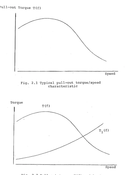
example, where several features must be considered. The typical pull-out torque/speed characteristics of a step motor are shown in Fig. 2.1. This represents the maximum

torque which the motor can develop at each operating speed. If the load torque

exceeds the pull-out torque, the rotor is pulled out of synchronism with the magnetic

field and the motor stalls or even reverses. However, for velocity profiling operations,

timing is critical, more factors have to be considered. Fig. 2.2 shows the relationship

between pull-out torque and load torque. It can also be algebraically expressed as

follows (Acarnley 1982):

Where, T(f) - the pull-out torque at a stepping rate f;

T 1 (f) - the load torque;

J - the whole system inertia;

8(t) - the rotating angle of the motor.

(2.1)

That means, to move the load and change its velocity at the required rate, the being

developed torque of the motor must be large enough to overcome the load torque and

accelerates the system inertia, thus to keep the consistent accuracy and stability, which

are the essential requirements in step motor control. Otherwise, the motor either fails

to operate at all or drops out of step during acceleration and deceleration, causing

permanent errors (Acarnley 1982; Dunlop 1986).

To perform each specified movement during a microprocessor software direct control,

can be calculated by knowing the step length. The former one can be obtained from

the following method based on the one of Acamley (1982).

The flowchart shown in Fig. 2.3 is the method giving the step interval by software for

direct control of one motor. At regular step intervals, the microprocessor software

produces a phase on/off pattern and sends it to the step motor phase switches. The

step interval can be calculated from the following:

Step Interval

=

+

Where, T 1 - the time taken to go through the idle path;

T 2 - the time taken to go through the step path;

d - delay value.

(2.2)

The step interval delay value d is placed in a loop counter initially, then the step interval

is established by decrementing the counter and producing a new phase on/off pattern

each time the loop counter reaches zero. Note that the loop takes typically lOllS per

loop cycle going through the idle path except on the last cycle which takes a typical

extra 50lls going through the step path. The addition of "DelayS" is to keep the time

taken in step path a constant no matter whether or not a new table is set up. The

"DelayL" here can be zero and must be increased in multiple motor control which is

discussed in the next section. Then the stepping rate can be calculated by the follo\\ring:

1

Step Rate (steps/sec)

=

The timing quantization is introduced by this microprocessor software loop. The effect

on performance is illustrated by the calculated results given in Table 2.1 (Dunlop and

1) The maximum speed a motor can achieve may be limited by the operating speed

of the microprocessor to less than theone determined by the load.

2) At high step rates, the velocity changes (or acceleration) which must occur within

one step time (so as to maintain synchronism) are very large. For every 10 times

increase of the speed, the required acceleration increases 1,000 times. In other words, a large torque is required to achieve large speed change when the speed is high; while a

small torque is required to achieve small speed change when the speed is low.

Nevertheless, this is contrary to the pUll-out torque/speed characteristic of a step

motor. That is, the torque T(f) available from the motor is greatly reduced when the

acceleration required to achieve the speed change is largest at higher speeds (c.f. Fig.

2.2). At slow speeds, the acceleration is much less and the torque available is much

greater. A software based microprocessor system can give satisfactory control of the

velocity profile up to stepping rates of 10,000 steps/sec, but may limit high-speed

performance (Acarnley 1982).

The use of a faster microprocessor to reduce the loop and calculation times will

increase the upper speed limit and reduce the differences between velocity changes

within one step time. However, in the final analyses, the inherent timing quantization

rather than the potential motor performance limits the control of the motor speed

predominan tl y.

3) The speed resolution decreases as the speed increases. For example, at 100

steps/s, a unity change in step interval produces a 0.1 % change in stepping rate, but at

2.3 MULTIPLE MOTOR CONTROL PROBLEM

The method of direct control of more than one motor by a single microprocessor is

shown in Fig. 2.4 (Dunlop and Ma). The DelayL shown in Fig. 2.3 must be increased so that the time taken in any motor control block is a constant irrespective of whether

the step output or idle loop path is taken through the flow chart. If this is not done,

then the 50lls overhead for the [lISt motor's step generation can occur anywhere within

the timing loop for the second motor (Dunlop 1986). This causes a variation in the

stepping rate of the second motor, which in tum affects the stepping rate of the first

motor. The effect of introducing a 60 Ils (50+10) loop delay for each motor is

calculated in Table 2.2. The figures are for a typical microprocessor controlling six

motors. Compare with Table 2.1 and it will be seen that the three problems associated with direct motor control of one motor are greatly multiplied for six motors:

1) The maximum velocities attainable are reduced, for the example in Fig.2.3, the

velocity drops from 16,667 to 2,778 steps/so

2) High acceleration is required at lower speeds. The upper speed limit given in

Table 2.2 for six controlled motors is 2778 steps/sec. The same acceleration required

(1.9E6) to reach this speed would produce a single motor speed of about 5600

steps/sec, or more than double the six motor control speed limit. Allowing for an

approximate halving of the torque for a doubling of the speed, then a torque limit of

1E6 yields a single motor speed of 4545 steps/sec or a 60% increase in the speed

possible with six motors. To achieve the same upper speed limit of 2778 steps/sec, the

single controlled motor requires acceleration of only 2E5 or 10% of that required for

six directly controlled motors. This has a large effect on the choice and cost of the

motors. In Fig. 2.5, Curve 1 shows the torque required to achieve the acceleration

When the motor speed is above 006' which is lower than WI' the torque will not be

sufficient to achieve the speed change.

3) The speed resolution is reduced further. Compare the calculated values given in

Tables 2.1 and 2.2. A speed of say 2020 steps/sec must be achieved by operating at

the nearest attainable step rates. For direct control of one motor, the attainable rates are

2,000 or 2,041 steps/sec whereas for six motors, the rates are 1,389 or 2,778. The

percentage speed change available at rates of 100 and 1000 steps/sec are 3.7% and

50% for six controlled motors compared to 0.1 % and 1 % for a single motor.

By using six microprocessors each to control one motor, these problems can be

lessened but only with increased cost and bulle.

2.4 ACCURATE MULTIPLE MOTOR CONTROL

The solution to the problems mentioned above is to use one dedicated controller with

microprocessor functions per motor so as to achieve the performance typified by the

values in Table 2.1. The addition of an encoder disk permits closed loop controL In

particular, the time between steps is then set by the movement of the rotor rather than

by a timing loop. While the time taken for the rotor to move is not quantized, the time

at which the encoder is sampled by the microprocessor is still quantized. However,

closed loop control prevents the loss of synchronism so that the previous requirement

that the velocity change occurs within 1 step can be relaxed and acceleration

requirements reduced.

The control requirements for a single motor have been incorporated in special VLSI

circuits from a number of manufacturers. The HCTL-1000 (c.f. Fig. 3.4) made by

general control of hydraulic cylinders and DC motors. Units such as the LM628 from

National Semiconductor can give full 32 bit PID control of DC motors and hydraulic

cylinders. Other units such as the Intel IDD008 or the cybernetics Micro systems

CY512 provide direct open loop control of a step motor. The HP unit met the

requirements for a general purposed Stewart platform controller and is readily

available. The 24 bit position accuracy is sufficient for most purposes so the HP unit

Pull-out Torgue T(f)

Fig. 2.1 Typical pull-out torgue/speed characteristic

Torgue

T(f)

Fig. 2.2 Pul out torgue T(f) and load

torgue T

1(f) characteristic

Speed

Set up Tables:

Count <-- No of Time Intervals NoReq <-- Step No Required

Set Directions Motor Control Block

...

~

... .

.

;I'

Step Path 50j.Ls Idle Path lOj.Ls

(DelayL=O)

NoSteps <-- NoSteps+l Rotate Bit Pattern Left

=

+

NoSteps <-- Nosteps+l Rotate Bit Pattern Right

No of Time Intervals <-- NewHo NoReq <-- New NoReq

Set Directions

output Bit Pattern

Count <-- No of Time Intervals

Count <-- Count-l

.

< l . " ' q , . I & • • • • 1 I 0 1 i t • • • • • O O o ; l O • • 9 • • • • • • 9 1 1 0 • • • • • • • 0 0 . Q I I I $ • • • • • • & o , . O • • • • • • •

Time Loop Time step Rate Speed Change eration

Intervals ,us steps/s steps/s steps/sis

1 2 3 4 5 12 13 14 15 16 17 18 29 30 31 32 43 44 45 46 94 95 96 994 99S

1*10+50=60 16667

2*10+50=70 14286 2381.0 3.4E+07

3*10+50=80 12500 1785.7 2.2E+07

4*10+50=90 11111 1388.9 1.5E+07

5*10+50=100 10000 1111.1 1.lE+07

.

.

12*10+50=170 5882 367.6 2.2E+06

13*10+50=180 5556 326.8 1.8E+06

14*10+50""190 5263 292.4 1. 5E+06

15*10+50=200 5000 263.2 1. 3E+06

16*10+50=210 4762 238.1 1.lE+06

17*10+50=220 4545 216.5 9.8E+OS

18*10+50=230 4348 197.6 8.6E+OS

·

·

29*10+50=340 2941 89.1 2.6E+OS

30*10+50=350 28S7 84.0 2.4E+OS

31*10+50=360 2778 79.4 2.2E+OS

32*10+S0=370 2703 7S.1 2.0E+OS

43*10+50=480 2083 44.3 9.2E+04

44*10+50=490 2041 42.S 8.7E+04

4.5*10+50=500 2000 40.8 8.2E+04

46*10+50=510 1961 39.2 7.7E+04

94*10+50=990 1010 10.3 1.0E+04

95*10+50=1000 1000 10.1 1.0E+04

96*10+50=1010 990 9.9 9.8E+03

·

·

994*10+50=9990 100 0.1 1. OE+Ol

99S*10+50=10000 100 0.1 1. OE+01

Table 2.1 Typical step rates and accelerations produced by direct microprocessor control of one step motor. The

set up Tables for Motors L .6

Set up Directions

I

I

I

I

~

.

•

l

I

I

Time Loop Time step Rate Speed Change Acceleration

Intervals ;\Is steps/s steps/s steps/sIs

1 1*60*6-=360 2778

2 2*60*6=720 1389 1388.9 1. 9E+06

3 3*60*6=1080 926 463.0 4.3E+05

4 4*60*6=1440 694 231.5 1.6E+05

5 5*60*6=1800 556 13B.9 7.7E+04

27 27*60*6==9720 103 4.0 4.1E+02

28 28*60*6=10080 99 3.7 J.6E+02

Table 2.2 Typical step rates and accelerations produced by direct microprocessor control of six step motors. The algorithms shown in Figs. 2.3 and 2.4 were used with

Torque

Curve 2

1

o

CHAPTER 3

DESIGN OF A MULTI-MOTOR CONTROLLER

3.1 INTRODUCTION

Running multi-axis machinery, fulfilling the above task required and obtaining good

performance at reasonable cost was the design principle of this whole system. The

whole structure of the control system completed during this research is schematically

shown in Fig. 3.1. The motor drives will be discussed in next chapter and the

performance of the system is examined in CHAPTER 5. In this chapter, the design of

a computer based six motor controller incorporating with six HCTL-1000 units is

discussed.

In view of present conditions such as computers, HCTL-IOOO units available

commercially and future development, a versatile controller was designed. It can

control one to six driving components. The driving components can be such as DC,

DC brushless and step motors as well as hydraulic cylinders. The controller can be

expanded to control more driving components with the same technique. The design

will be described in three parts: computer, HCTL-lOOO and the design of the

3.2 THE COMPUTER AND ITS I/O CHANNEL

The IBM Personal Computer is used very popularly. It has Intel 8088 16-bit microprocessor as .the Central Processor Unit. It has 16-bit registers and internal

operations but uses an 8-bit input-output and data bus. The address bus is 20-bit so

the maximum amount of memory that 8088 can address is 220 , or 1MB of memory. It

normally has 64 KB to 256 KB of RAM memory, 40KB ROM memory. It may have 8087 mathematics co-processor to increase the computing power of the machine. Also

it has 8 expansion slots which allows additional devices to be added on the system.

The 8088 runs on a4.77 to 8 (8088-2 CPU) MHz clock cycle. It also has a proper

and efficient Disk Operation System (DOS).

With so many features it was used as a card cage for the multi-motor controller Printed

Circuit Board and a programmer for the HCTL-lOOO motion control ICs. This

desktop computer was chosen for the extensive expansion bus hardware and software

support, as its memory and operation speed are enough in this application, plus its low

cost.

The Input/Output (I/O) channel of an IBM-PC is an extension of its Intel 8088

microprocessor bus. It contains an 8-bit bidirectional data bus, a 20-bit address bus (the top 10 bits are not decoded), I/O read and write, and some memory control lines.

These functions are provided via a 62-pin edge connector (c.f. Fig 3.2) which is also

called "expansion slot". There are 8 slots on the system board of an IBM-PC. The I/O

devices are addressed using I/O mapped address space. The channel is designed so

that 768

110

card, which is for users to design their own circuit to connect to the expansion I/O

channel of the microprocessor bus, occupies 32 spaces from 300-31FH. The

controller were allocated 12 (of 32) I/O addresses from 300H to 305H and from 308H

The functions of used I/O signals are:

i) AO-AII: Output. Can address 12 bit's I/O device. Logic high is 1. ii) 00-07:

iii) -lOR:

iv) -lOW:

I/O. Provide data bus bits 0 to 7 for the microprocessor memory and I/O devices. Logic high is 1.

Output. -I/O Read Command: This command line instructs an I/O device to drive it's data onto the data bus. Active low. Output. -I/O Write Command: This command line instructs an I/O device to read the data on the data bus. Active low.

v) AEN: Output. Address Enable. This line is used to de-gate the microprocessor and other devices from the I/O channel to allow DMA transfers to take place. Active high.

vi) RESET DRV: Output. Reset Drive: to reset or initialize system logic upon power-up. Active high.

3.3 THE HCTL-I000

The HCTL-lOOO is a high performance, general purpose motion control IC. It performs all the time-intensive tasks of digital motion control, thereby freeing the host processor for other tasks. The complete servo system is made up of a host processor to specify commands, an HCTL-IOOO to fulfill the algorithm, an amplifier and motor with an incremental encoder (c.f. Fig. 3.3).

3.3.1 The Operation

bidirectional multiplexed address/data bus interfaces the HCTL-IOOO to the host

processor. The encoder feedback is decoded into quadrature counts and a 24-bit

counter keeps track of position. The HCTL-lOOO executes anyone of four control

algorithms selected by the user. The four control modes are:

-Position Control;

-Proportional Velocity Control;

-Trapezoidal Profile Control for point to point moves;

-Integral Velocity Control with continuous velocity profiling using linear

acceleration.

More details are given in CHAPTER 5.

The resident Profile Generator calculates the necessary profiles for Trapezoidal Profile

Control and Integral Velocity Control. The imbedded microprocessor in the HCTL·

1000 compares the desired position (or velocity) to the actual position (or velocity) and

computes the error which is input to a programmable digital filter Dl (z). The filter

output provides compensated motor control in the form of an 8 bit DAC voltage. or a

Pulse Width Modulated (PWM) signal and direction signal. A commutator port can be

programmed to provide electronic commutation for brushless DC and step motors. Thus, by using such a comprehensive microprocessor, the step time quantization

problem can be greatly reduced.

3.3.2 User Accessible Registers

The HCTL-lOOO operation is controlled by a bank of 64 8-bit internal registers, 32 of

which are user accessible. These registers contain command and configuration

information. Only by accessing these registers, can users run the controller chip to

perform each required control functions. Fig. 3.5 shows the functional block diagram

3.3.3 Timing Diagram

The control bus of the HCTL-lOOO contains four I/O lines, ALE (Address Latch

Enable),

CS (Chip Select). OE (Output Enable) and

R!W

execute the data transfers between the registers and the host processor over the 8-bit

address/data multiplexed bidirectional bus. By satisfying a timing requirement, these

lines can execute data transfers.

There are three different timing configurations. The ALE/CS non overlapped timing

configuration was used upon the use of 8088 microprocessor in IBM-PC (c.f. Fig.

3.6),

To access data to or from the HCTL-lOOO registers. ALE (Address Latch Enable)

pulse is asserted flISt. This routs the external bus data into an internal address latch (so called "external" and "internal" are relative to the HCTL-lOOO).

'C'S'

latch. Rising'CS starts the internal synchronous process.

In the case of a write, the data in the data latch are written into the addressed location. In the case of read, the addressed location is written into an internal output latch. then

OE (Output Enable) low enables the internal output latch onto the external bus. Thus

3.4 DESIGN OF THE CONTROLLER

A six motor general purpose controller was designed during this research. The

schematic logic diagram is shown in Fig. 3.7. More illustrations in detail for each part

of it are given in the following subsections.

3.4.1 IBM-PC I/O Bus

The signals used to communicate with the HCTL-lOOO units come from IBM-PC I/O

bus (c.L Fig. 3.2). The signals are provided in a 62-pin expansion slot sitting on the

system board ofIBM-PC. The functions of them were illustrated in 3.2.1.

3.4.2 Decoder and Control Logic

This part decodes all address and data accessing commands from the host processor

and controls the correct timing.

3.4.2.1 Clock

The diagram of the external clock is shown in Fig. 3.8. A 3.6864 MHz crystal was

used as an oscillator. A DM74 109 Dual J-K Positive-Edge-Triggered Flip-Flop was

used to generate square clock output at frequency of 1.8432 MHz. The clock output

Pin 6 of U3 (abbreviated as P6/U3, same with others from now) goes to Pin 34 of each HCTL-lOOO unit to generate the processor control timing and to be used when

setting the sample period. Synchronism between the host and the slave processors is

The four control signals CS, R!W and are decoded shown in Fig. 3.9 in details. U4 is a 74LS688 Magnitude Comparator which compares bit for bit two 8-bit

words and indicates whether or not they are equal. One word is fixed as 30H by

connecting each bit respectively to Vcc or GND. Another word is input from the

microprocessor address bus All-A4. When an I/O address having XX30XH pattern

is input via the 20-bit I/O address bus (NB: X not care), the middle part of it 30H

will match the fixed word, so the Pin 19 of U4 is selected (goes low).

Note that the signal AEN (Address Enable) in IBM-PC I/O bus is used here to disable

the Pin 1 of U4. The AEN is a DMA (Direct Memory Access) control signal. When

this line is active (high), which happens regularly for memory refresh, the DMA

controller will take over the control of all the address bus, data bus and control lines to allow DMA transfers to take place. Because DMA also communicates with liD

devices, the active high DMA interrupt regularly appears on the expansion bus. This

will disturb the decoding logic of the controller. Thus AEN must be used so that no

I/O addresses in the six motor controller tan be selected when the AEN is taking place.

U5, U6 and U7 are 74LS 138 DecoderslDemultiplexers which decode one-of-eight

lines, based upon the conditions at the three binary select inputs (Pin 1-3) and the three

enable inputs (Pin 4-6). lORD and IOWR from I/O bus are used directly or decoded

through a series of gates to give R/W signal for the HCTL-lOOO.

If IOWR, address XX30XH (from Pin 19 of U4) and one of the addresses 8H to DH

(from slot pins AO-A3) occur and are input into input pins of U7 respectively, U7 will

provide an output signal to Pin 38 of an HCTL-IOOO unit. If IOWR or lORD,

address XX30XH and one of the addresses OH to 5H occur, U 5 will provide to

8H-DH are written, U6 will provide OE to Pin 40 of an HCTL-lOOO unit. Thus the tinnng requirement by the HCTL-lOOO is satisfied.

The addition of the capacitor C3 is to delay the falling edge of to ensure it happens a minimum period after the rising edge of CS as required, therefore, the data output from the internal location of the HCfL-lOOO into its internal output latch are valid.

3.4.2.3 Data transfer

U8 is a 74LS245 Tri-state Octal Bus Transceiver. When Pin 19 goes low, which means one of the I/O addresses from 300H-30DH used is selected, the data on one side of the U8 can be transnntted to the other side depending on write or read. cycle If the data are read into ffiM-PC, the Pin 1 goes low, the data on the HCTL-lOOO's data bus will be transmitted to the ffiM-PC data bus. In the case of writing data to the HCTL-lOOO, Pin 1 keeps high, then the data on the IBM-PC I/O data bus (DO-D7 in slot) will be transmitted to the data bus of the HCTL-lOOO units (Pin 2-9).

3.4.2.4 An example

An example is taken to explain the functions of the Decoder and Control Logic, combining with software program written in assembly language. A number 83H, for instance, is to be placed in the HCTL-lOOO's internal register R20H and a number is to be read from. Table 3.1 shows the whole procedure.

S 1 is mounted. The Reset signal received by the HCTL-IOOO will lead to a reset of

internal circuitry and a branch to Reset mode.

3.4.4. HCfL-lOOO

Six HCfL-1000 units are used each for driving one motor. PWM and its SIGN

signals are used for driving DC motors. Some provision were made for driving other

types of driving components, i.e., PHA-PHD and INDEX signals are led (c.f. Fig.

3.11).

Except 4 control lines, 8 bit address/data, Clock, Reset are received by each

HCTL-1000 to process the algorithm, total 12 signals are led from each HCTL-lOOO unit.

The 12 signals are:

i) PULSE (Pin 16) - Pulse Width Modulated signal. Output. The duty cycle is proportional to the Motor Command magnitude and is used for a DC

motor or hydraulic cylinder speed control signal;

SIGN signal (Pin 17) - Output. Gives the sign/direction of the pulse signal

ii) PHA-PHD (Pin 26-29) - Output. Four commutator signals to provide phase switching infoffi1ation to step or DC brushless motors;

INDEX (Pin 33) - Index Pulse, input from the reference or index pulse of an

incremental encoder. Used only in conjunction with the Commutator.

iii) INIT (Pin 13) - InitializationlIdle Flag. Output. This is a status flag indicating

that the controller is in the InitializationlIdle mode.

iv) (Pin 15) and LIMIT (Pin 14): Input. Internal flags set externally. A

manul LIMIT switch is mounted beside the Stewart platform for use in

the case of emergency (cL Fig. I), Once the LTh1IT flag is set in any control mode, it causes the HCTL-lOOO to go into the Initialization/Idle

Mode, clearing the Motor Command and causing an immediate motor

v) CHNCHB (Pin 31/30): Channel A, B - Input pins for position feedback from

an incremental shaft encoder. Two channels A and Bare 90· out of phase which will give the counter of the HCTL-lOOO quadrature

position input and also give direction infonnation.

3.4.5. Buffer

Each of the Input/Output signals of the HCTL-lOOO units is buffered by a channel of a

74LS244 Octal Tri-state Buffer, which provides improved noise rejection and high

load drives (c.f. Fig. 3.12),

3.4.6 Contro11er Socket

A 96-pin connecter is soldered on the controller PCB, which is inserted on an

expansion slot. The signals are shown in details in Fig. 3.12 and go to the motor

drives through cables.

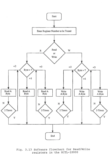
3.5 Testing and Debugging

A general purpose testing program was written and used to access every register inside

the HCTL-IOOO when debugging. The flowchart is shown in Fig. 3. 13.and the

---3 x 2-MOTOR

DRIVER

FEEDBACK UNES FROM MOTOR SHAFT POSITION ENCODERS

Fig. 3.1 Schematic structure of the control system for stewart platform

W

Rear Panel

Signal Nam e _\ Sig nal Name

GNO r -

t-81 AI- r - - -110 CH CK

*

-

• 5V _!-

-

.IR02 _!-

-

-SVDC -

-

*

.DR02 _!-

-

-12V _t-

-

-CARD slew _I-

-

'IlV _{I -}

-

GNO I-810 1\10 .110 CH ROV

-MEMW _t-

-

*

-M£MR _I-

-

*

-

*

-

-DACKl _I-

-

.OROl _I-

-

-OACKI _t-

-

-

---

.DROI

~

-

-DACKO I-

-

elK I-820 1120 - tAil

.IRDI _{I -}

-

'IAO&

-

-

'IAOS

-

-

.IRD4

-

-

.IROJ

-

-

*

-GAUl _-

-

-

• TIC

-

-

'ALE _I-

-

'5V i--

-

-OSC I-

-

.GNO i--6JI All

-'--- '--- 'M

\

Fig. 3.2 IBM-PC computer I/O channel diagram

Host Processor

HCfL~1000

ADO/DBO ADIIDBI AD1/DBl I\OJ/DDJ

1\04/DD 4 1\06 /DB 5

r

I

- r

I

:

:-

I

--.--

I

I

I SAMPLE

I

,

--

I

I

L_

----POSITION

I

,

cv

-- -

----CHA CHB

EMERGENCY FLAGS D,IZI DIGITAL FILTER t

PROF INIT

---

--

---,

I

I

FLAGS

MOTOR COMMAND

PORT

I

COMMUTATOR

I

l

:

I I I

l

I

l

-

- - -

---

Fig. 3.4 HCTL~1000 internal block diagram

Fig. 3.5 The HCTL-IOOO register functions

~AI "}\I

'~-Ai

''AI

fi\!.

"Afl\~~cepi i~"i'~:li1n~i

{pi6~'cirtioh'~I\j~'lol ;AI,I::1;::~}:!;[{~~\{:;~1!i;j!~:!!:~

Propbrtiq"al,Veloc ',,'

'Ptoportkiri1i1 \/elocliy;;:~;:

i

iriiegrai.\}elochY" arid

iTrape~6jdaIProf!leii:

,iniedfaliVelodty,'sn

" .

l.rrrapeioldal'prOflle;

';;rrapezo!dal: Profile : scafa~15J

'~tr~pez6IdaIP~Clfile, ,,',;. ,,'lf1 .2'sco'nipI9

rn

;;Trapeiol?arRro!'tie'ri;:«(f:;;):l~:~j~ i,~?:s'cproPlerh~h~ ~Trapezoidat:f'wljle ;'{;'," ":~y:~:s;pbfT)plernent

I :'EroP()~!ona,\;~el~:C!ty;N;;2:S;'fompi,en,1~ni;;:j;'

,f~OportloraIVet9clty !A;2~.scofT)pl~fT)el1!:

;,ht'eg;~I:\ielocity),1;;;,i:';;;;

2'5

conip1ement:}.f

~~~~~~~~~~~~~~~~~~~~~~~~~ ~~~~~--~~~~~~~~~~~

Noles:

1. 'Upper4 bils are read only. ., ;;"{'':'''':'<''; , j I I: 2. Writing to ROEH (lSBI lalches all 24 bils. ';.:'" ' . '" 3. Reading A14H (lSB) latches data inlo A12H and RI3H,

I ' ..

" . , • ,', ~ " • I , 1 , ; : " -:'

4. Writing to Rl3H.clears Actual Position Counter to zero .. The scalar data is limited to positive numbers (DOH to 7FHI. 6. The commutator regislers IRI8H, RICH, R1FHl have further limit

. which are discussed in the Commutator section of this data sheet.

Write Cycle ALE

CS

R/W ______________ ~~ ______ ~ ________ __

.:xxx

~

YJYY.X.li:'!J$i

Read Ie

R/W

OE

lX:lX

x:x:xxxxxxxxxxx

X2K

~ I D M

I

~O-A.ll ALEl PWH PWI1

12 2 2

'fOTffi DEI PHA-

PHA-J PHD PHI)

IOWR CSl HCTL- 4 4

1000 CHA- Buffer CHA- Motor

00-07 _{R/W CHB CHB 1}

8 unit 1 2 2 Drive

STOP SToP

Decoder _I LIMIT LIMIT

I

"

,

control

.

.

Logic

I A'LE6 Plm PWH

OE6 PHA-

PJlA-3 PHD PlIO

I CS6

HCTL-1000 CHA- Buffer CHA- Motor

l&[ CnB CUD 6

unit 6 DriVe

Clock STOP STOP

2 MHz

/

B Bit Bus

Each chip is accessed by J decode lines ALE, OE and

cs.

300n CS1, read or write unit 1; J05H Cs6, read or write Unit 6.

JOBH ALE1, write the register number selected JOOH ALE6, write the register number selected JOSH OE1, read the output buffer of unit 1; JODH OE6, read the output buffer of Unit 6.

Fig. 3.7 Computer and motor interfaces for the motor controller

~---~'DI~---~

U1E 3686.4KHz. UiD

74LS1-4

Ai it<

8

74LS1-4· R1

it<

PINS 1.2. l5. 11. 12. 13. 1.4. 15.16 TO +5V

U3A

to Pin 34 of HCTL-lOOO units

7

DH74109

Fig. 3.8 Clock diagram for the motor controller

¢ .

signals

pC-XT

I

1

OARO

- lOR fl14

- row

i\~FlN All A4 A3 AO DO D7 A11 ;1..20 A21 A2ii! ;'23 ;1..24 ,0.20 ,o.2t1 1'.27 A2S A29 A30 A31

V

?'La,. ' ] ?'La" 74LB1~

100nr

1~

:2 )

:"I

"'-",UOO

U.<I

1 .1

1~ G P-Q "1

-9- Q4 P-4

v~c

34 Q3 P3 1

=1

~ ~

Ptl 06

P2 G2

1 01 ₀₇ P1 _P7 1

cao PO

'" Sff&s -=~

;

-ofHCT L-IOOO

'l~m1~tnn:lr~T

111'1

I')

1326 V7

-4'

tl 52A _1>1 't6 _VO

't'"

3 V3

<' C Y2

~ .e _A 't,1 _VO

'141..'" 13S

~

~ :"I Jf--~"--300H pins TL-IOOO to CS

of HC

OUTPUT ENAEfCr

us

15. _{e2t} V7}

t

.oj:

fi' e;:;A V6 ~

GJ. YO 30DH

Y4 V3

3

<' C 1 fl.

V2 P.

V1

-308H pin s 'L-IOOO

".

74UH38 to OE of HC'!

~~

U7

1'\, G2f1 _V7

.c' _{G2,o. YB}

6"

131 ye

Y4

3 Y3

<' C Y2

1 6 '1'1

A YO

'''LIHsa

APOR/DATA

us

PIR e

Ai 1:11

... 2 62 AS 1:13

,1.4 a ..

;'0 £10

;'6 as

A7 67 AS Be

74LS24I~

,

~

:.:

~--308H E pins L 1000 to AL

ofHC'l'

flua

---to data bus of HC'l'L-IOOO

Table 3.1 An Example - write Data to and Read from HCTL-1000

Function Program IBC-PC Interface HCTL-lOOO U14

Write 83H LDA, 20H IOWR is generated ALE (on Pin ALE(on Pin 38) into register OUT (308H), A on I/O bus, 15 of U7) IS gIVen

20Hin Address 308H occurs

HCTL-lOOO appears on I/O

U 14 bus AO - All;

20H appears on which enables low

I/O bus DO - D7 6 bits (20H on Pin

2-7) of external data bus into internal address latch

LDA,83H IOWR is generated CS (on Pin CS (on Pin 39)

OUT (300H), A on I/O bus, 15 of U5) IS gIven,

Address 300H occurs R!W (on Pin 37)

appears on I/O is given

bus AO-All;

83H appears on The external data bus

I/O bus DO-D7 data (83H on Pin 29)

is written into the internal address location

(Table 3.1 continued)

Read a LDA,20H lOWR is generated ALE (on Pin ALE (on Pin 38) datum from OUT (308H), A on I/O bus, 150fU7) is given,

register Address 308H occurs

20Hin appears on I/O

HClL-lOOO bus AO-AIl;

U14 20H appears on Which enables low

I/O bus 00-07 6 bits (20H on Pin 2-7) of external data bus into internal address latch

IN A, (300H) lORD is generated CS (on Pin CS (on Pin 39) is on I/O bus. l50fU7) given,

Address 300H occurs R (on Pin 37) is

appears on I/O given,

bus AO-AII; Data is read from an

internal location into an internal output latch

IN A, (308H) IORD is generated OE(onPin R on Pin 37) is given, on I/O bus, 150fU6) OE (on Pin 40) is given Address 308H occurs which enables the data appears on I/O in the internal output

bus AO-All latch onto the external

data bus to complete a Read operation The data to be

PC bus Reset Drv

B2

from

Decoder ~

and

---7

Control Logic A03/DB3 ,1.0<1/013<4 AOEl/DBB 086 OB7 EXCLK ADO/BOO AD1/0B1 A02/082 "'03/083 A04/08-4 A0I5/0BI5 0136 DB7 EXCLK AOO/BOO AOS/OB1 A02/082 AOS/OB3 AO"'l/OB<4 A0I5/0815 OElf! 0137 EXCLK ADO/BOO A01/0B~ A02/0B2 A03/0B3 "'0<4/013"1 "'015/0136 DBB OB7 EXCLK ADO/BOO ADS/OBi "'02/0B2 "'03/0B3 "'04/0134 "'015/01315 Dee OB7 EXCLK "'DO/BOO AOi/0Bi AD2/0B2 "'03/063 A04/0B4 A0I5/0615 OBS OB7 o

PUL BE SIGN ....

!-tZ=====

PHB I-§~--­

CHBk~--­

CHAI-"'CiL..---diffi-

~f----PHS

Hli:-k----PHC

HP<'*----PHD I-!ii~--­

CHB

H<'¥----

~~--tim·~

PULSE

I-+-~---8X GN ~",---­

PHO-

~~--INIT ~*---­

PHA

Hii*----PHs Hii-k---~ PHC:~~--­ PHO~¥---­

CHB~·¥---;'"

~

b-/-"<----Fig. 3.11

HCTL-1000 input

and output signals

_C4 ₄₉

B4

!;1

--

-"-'I

'"

=i!

A

:,1,3 _ _ _ t>=><:=>_"'="t=Io>=O"'""'C>mI>'"""""""""' ... _

PHA PHE! SIGN i

~ INDEX ElTOP PHD 2

0

M _{PHC eHS CHA :3}

_c~

_C3 ~ INI1' LIMIT PULSE

'"

11.2

-C2

----~---~---ea

-CI5 PHD eHA +15V 15

-ElI5

~

:ce

PHC STOP oIoi5V 7

44 M

a

LIMIT PHA +ElV 9

:gg

_ _ 67

-_C~O PHD CH ... +I5V 11

Ell;

:B10

§

_ _ C7

_Be _M PHC STOP +!5V 13

i

LIMIT PHA +eIV :1.15 _C14

_C1!5 PULSE PHa +I5V 115

:g~~

---_CU PHD CH" GRND :1.7

_ _ 8S'" _811

~

_C12

from _M PHC STOP GRND 19

HCTL-1000 U INIT CH8 SRND 20

~ LIMIT PHA GRND 21

_1313 PULSE PH8 GRND 22 _CHI

_8:1.2

---~---_8Sfl PHD CH.&. !!lRND 2:3

_82~

_822 _~ INDEX SI!!lN ORND 24

_ca9

~

i

LIMIT PHA !!lRND 27 PULSE PHe GF'lND 2e

1A2 1'(2 _C20

---~---2'(2 2,6.2 _C2S

2V3 2"3 _819 ~ PHD eH" SI!!lN 29

1A4 1V"I _C22

1"3 1V3 :~i~ 0 M INDEX STOP PHe 30 1A1 1'(1

2V,,", 2""'1 _820

l

2Y1 2,6.1 _Cie _{INIT LIMIT PULSE :32}

4 s 44

--_

_-_

_-"""""--C 8 A _C2B

_927 _929

_C2!3 PIN ASSIGNMENT

_C23 _926

_923 gS-PIN CONNECTOR ON PCB

_C2A1

Fig. 3.12 Buffer and

_1::27

_B2E!

_C29 _{controller socket diagram}

_B 2 "'I

_C:31

Read A Byte

=2

=1

Read A Byte

Start

Enter Register Number to be Tested

R

=3

Read A Byte

Write A Byte

W

=2

=1

Write A Byte

Fig. 3.13 Software flowchart for Read/Write registers in the HCTL-IOOOO

=3

CHAPTER 4

DC MOTOR PWM SERVO DRIVE

4.1 INTRODUCTION

The Stewart platfoID1 proposed in CHAPTER 1 has six legs driven by six actuators.

Several types of actuators, such as hydraulic cylinders or various types of electric

motors, could be chosen. Hydraulic cylinder linear actuators, which convert hydraulic

power into linear mechanical work, are the best choice in this high precision and heavy

duty control application due to their fast dynamic response, good mechanical stiffness,

large force capability and high power. Unfortunately, they are also expensive and thus

were not used at this stage of the project.

The DC motors became the next best choice owing to their outstanding advantages: They provide a wide variety of operating characteristics obtained by selection of the

excitation method of the field windings. Also they provide ease of speed control, high

efficiency, the conditions of high torque and low voltage, and are relatively

inexpensive. In this research, six Electrak 100 Linear Actuators driven by peID1anent

magnetic DC motors were chosen (cLWarner Electric Catalogue 1985).

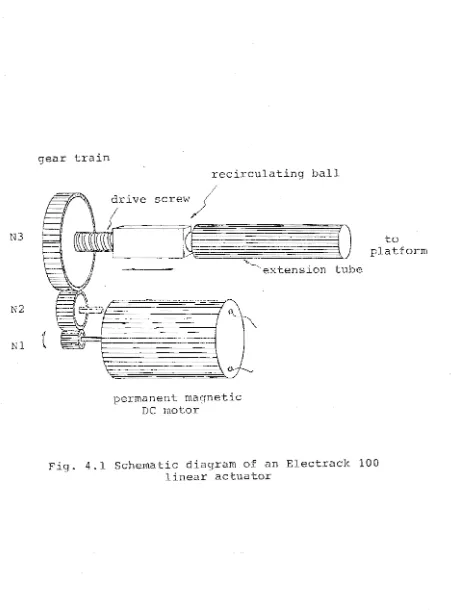
The principle of operation of the actuators is shown in Fig. 4.1. A drive screw and a

recirculating ball covert the rotating movement, transmitted from the motor via the gear

train, into linear movement, so that the extension tube (the leg of the Stewart platfoID1),

The parameters of the EleclTak 100 linear actuator are: SlToke length 24"

Pitch of the screw 0.2" Gear train: N1= 16

N3= 80

Gear lTain ratio 1:5

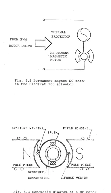
The permanent magnet DC motor in the actuator is shown in Fig. 4.2 (c.f. Warner 1985). There is a thennal protector inside of the motor housing, which protects the motor from overheating.

The overview of various DC motors, particularly the permanent magnetic DC motors, which has good characteristics for speed conlTol, will be given in next section.

4.2 DCMOTOR

4.2.1 Operation Principles

The DC motor is basically a torque transducer. The torque is produced by the net force from all conductors acting over an average radial length to the shaft center (c.f. Fig. 4.3). The DC motor's characteristic is expressed in a linear relationship: the mechanically developed shaft torque of a DC motor is directly proportional to its armature current as the following:

Where, Tm - the shaft torque in Newton-meters;

<I> the magnetic flux per pole in webbers; Ia-the annature current in amperes;

E1>

When the conductor moves in the magnetic field, an induced voltage or back

electromotive force (emf) is generated across it, tending to oppose the current flow

through the conductor. This voltage is proportional to the shaft velocity:

(4.2)

Where E - back emf in volts;

ro - velocity in radian/second.

In a motor, the back-emf voltage E, plus the voltage drop Ia Rathrough the annature

due to annature current Ia and annature resistance Ra. must be overcome by the total

impressed voltage V m at the tenninals. The voltage relations are expressed by Eq.

(4.3):

(4.3)

Where, V m - terminal voltage in volts; Ra - armature resistance in ohms.

Equations (4.1), (4.2) and (4.3) form the fundamental basis for DC motor operation

(c.f. Fitzgerald 1983).

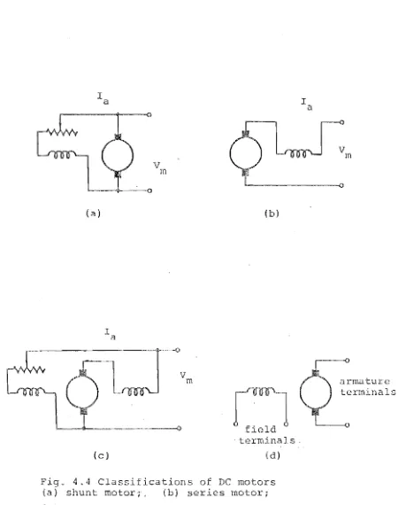
4.2.2 Classification and Characteristics

DC motors may be categorized as shunt, series, compound and separately excited

The field circuit and the armature circuit of a DC shunt motor are connected parallel

(c.f. Fig. 4.4 (a». The field current and pole flux are essentially constant and

independent of the armature requirements. The torque is therefore essentially

proportional to the armature current (c.f. Eq. (4.1»).

In operation, decreases in speed and back emf E, due to added load, produces an

increase in the small portion of voltage drop Ia Ra(c.f. Eq. (4.3». Since terminal

voltage V m is constant, Ia must increase some hence the output torque increase some to

give extra torque required. This produces a wide range of speed and torque

characteristics and the speed-load curve is practically flat (c.f. Fig. 4.5), resulting in

the term "constant speed" for the shunt motor. Typical applications are for load

conditions of fairly constant speed.

4.2.2.2 Series motor

The field circuit and the armature circuit of a DC series motor are connected in series

(c.f. Fig. 4.4 (b»). The flux of a series motor is nearly proportional to the armature

current Ia which produces it As a result, the torque of a series motor is proportional to

the square of the armature current, visa versa, large increase in torque may be

produced by a relatively small increase in armature current (c.f. Eq. (4.1).

In operation, the increase in load causes a decrease in rotor speed, hence a decrease in the back emf Due to decreased E, the armuture current must increase to provide

more torque to drive the increased load. This produces a variable speed characteristic.

The speed-load curve is the markedly dropping one shown in Fig. 4.5. The

4.2.2.3 Compound motor

A compound motor has two field windings. One is connected in parallel with the

armature circuit; the other is connected in series with the armature circuit (c.[ Fig.

4.4(c». With both field windings, this motor combines the effects of the shunt and

series types to an extent dependent upon the degree of compounding. This motor is

used when high starting torque and somewhat variable speeds are required.

4.2.2.4 Separately excited motor

The field winding of this motor is energized from a source different from that of the

armature winding (c.[ Fig. 4.4 (d», so that the two impressed voltages can be varied

independently, thus produces a wide range of speed and torque characteristics. The

required field current is usually a very small fraction of the rated armature current

(Fitzgerald 1983). A small amount of power in the field circuit may control a relatively

large amount of power in the armature circuit. Separately excited generators are often

used in feedback control systems when control of the armature voltage over a wide

range is required.

4.2.2.5 Constant field and permanent magnetic DC motor

Above four categories may all have variable magnetic flux. If the field excitation of a separately excited field motor is constant, the motor becomes a constant magnetic flux

one. More particularly, when the motor is small, it can be made with permanent magnet field with armature excitation only, which produces constant flux. The

permanent magnet field motor (c.f. Fig. 4.2) is described and highlighted in this

During the operation of a separately excited constant field motor or a permanent magnet

field motor, the field flux is constant and Eq. (4.1) simply becomes

Where, K_t is the torque constant of the motor;

and Eq. (4.2) becomes:

E::::::K ro _e

Where, Ke - back emf voltage constant

(4.4)

(4.5)

Note that, the mechanically developed power Pm must be equal to the electrical power absorbed in the rotor P e' i.e.,

Pm :::::: T m ro :::::: K_t Ia ro Pe=EIa=Kero1a Pm=Pe

Therefore, in MKS system, K_t :::::: Ke'

(4.6) (4.7) (4.8)

As can be seen, the relationship between armature current, torque and velocity is

simply linear. This simple mathematical relationship gives the ease of control in

incremental motion servo systems. However, the permanent magnet field motor has

more advantages over the wound field structure one. Firstly, there is no power

dissipated in the permanent magnet field. Therefore, the permanent magnet field motor

is more efficient and requires less space. Secondly, due to the availability of

permanent magnets with high coercive force characteristics, the linear relationship of

their wound field DC motor counterparts. Thirdly, the more simple structure of

permanent magnet field motor has more simple relationship between electrical input

parameters and mechanical output characteristics. This is why the permanent magnet

DC motor is very popular for use in motion control servo systems. The servo

calculations and system design of this application are discussed in CHAPTER 5.

4.2.2.6 Motorpararneters

Other parameters and characteristics of this permanent magnet motor in Electrak 100

are:

Current Draw: 9.1 Amps at 24VDC - 2.2kN (500 lb) capacity at fun load. Fig.

4.6(a) shows the specification of the