Partitioning the Intrinsic Order Graph for Complex Stochastic Boolean Systems

Partitioning the Intrinsic Order Graph for

Complex Stochastic Boolean Systems

∗

Luis Gonz´alez

Abstract—Many different problems in Engineering and Computer Science can be modeled by a complex system depending on a certain numbern of tic Boolean variables: the so-called complex stochas-tic Boolean system (CSBS). The most useful graph-ical representation of a CSBS is the intrinsic order graph (IOG). This is a symmetric, self-dual diagram on2n nodes (denoted byI_n) that displays all the bi-naryn-tuples in decreasing order of their occurrence probabilities. In this paper, two different ways of par-titioning the IOG –with applications to the analysis of CSBSs– are presented. The first one is based on the successive bisections of this graph into smaller and smaller equal-sized subgraphs. The second one consists of decomposing the graph I_n into totally or-dered subsets (chains) of the set {0,1}n of all binary n-tuples.

Keywords: complex stochastic Boolean system, intrin-sic order, intrinintrin-sic order graph, graph bisection, chain cover

1

Introduction

This paper deals with the analysis of those complex systems depending on an arbitrary number n of ran-dom Boolean variables. That is, the n basic variables

x1, . . . , xn of the system are assumed to be stochastic,

and they only take two possible values, either 0 or 1, with basic probabilities

Pr{x_i= 1}=p_i, Pr{x_i= 0}= 1−p_i (1≤i≤n). We call such a system acomplex stochastic Boolean sys-tem (CSBS). Each one of the 2n possible elementary states associated to a CSBS is given by a binaryn-tuple

u= (u₁, . . . , u_n)∈ {0,1}nof 0s and 1s, and it has its own occurrence probability Pr{(u₁, . . . , u_n)}.

Throughout this paper we assume that the n Boolean variablesx_i are statistically independent, so that the oc-currence probability of a given binary stringuof length

∗_{Manuscript received March 14, 2010. This work was partially}

supported by the Spanish Government, “Ministerio de Ciencia e In-novaci´on”, “Secretar´ıa de Estado de Universidades e Investigaci´on”, and FEDER, Grant contract: CGL2008-06003-C03-01/CLI.

†_{University of Las Palmas de Gran Canaria, Research Institute}

SIANI & Department of Mathematics, Campus de Tafira, Univer-sidad de Las Palmas de Gran Canaria, 35017 Las Palmas de Gran Canaria, Spain. Email: [email protected]

ncan be easily computed as

Pr{u}=

n

i=1

pui

i (1−pi)1−ui for allu∈ {0,1}n, (1.1)

that is, Pr{u}is the product of factorsp_iifu_i = 1, 1−p_i ifu_i= 0.

Example 1.1 Let n = 4 and u = (0,1,1,0) ∈ {0,1}4. Suppose that p₁ = 0.1, p₂ = 0.2, p₃ = 0.3, p₄ = 0.4. Then using (1.1), we have

Pr{(0,1,1,0)}= (1−p₁)p₂p₃(1−p₄) = 0.0324. The behavior of a CSBS is determined by the ordering between the current values of the 2nassociated binaryn -tuple probabilities Pr{u}. Computing all these 2n prob-abilities –using (1.1)– and ordering them in decreasing or increasing order of their values is only possible in prac-tice when the numbern of basic variables is small. For large values ofn, we need alternative procedures to com-pare the binary string probabilities. For this purpose, in [3, 4] we have established a simple positional criterion that allows one to compare two given elementary state probabilities, Pr{u},Pr{v}, without computing them, simply looking at the positions of the 0s and 1s in then -tuplesu, v. We have called it theintrinsic order criterion

(IOC), because it is independent of the basic probabili-ties p_i and it is exclusively determined by the positions of the 0s and 1s in the binary strings.

The intrinsic order relation on{0,1}n can be graphically illustrated through theintrinsic order graph(IOG). This is a fractal, symmetric diagram that scales all the 2n bi-naryn-tuples (associated to a CSBS with n basic vari-ables) by decreasing order of their occurrence probabili-ties.

describe the practical interest of the two different ways of partitioning the IOG, presented in the two previous sections.

2

Some Previous Results

Let us fix some basic concepts and notations, that we shall use in the rest of the paper.

Definition 2.1 Let n≥1 and let u= (u₁, . . . , u_n)be a binaryn-tuple. Then

(i)We indistinctly denote the n-tupleu∈ {0,1}n by its binary representation(u₁, . . . , u_n) or by its decimal rep-resentationu₍₁₀, and we use the symbol “≡” to indicate the conversion between these two numbering systems, i.e.,

(u₁, . . . , u_n)≡u₍₁₀ =

n

i=1

2n−iu_i.

(ii)The Hamming weight(or simply weight)w_H(u)ofu is the number of1-bits inu, i.e.,w_H(u) =n_i=1u_i.

(iii)Letu= (0, . . . ,0), i.e.,w_H(u) =m >0. The vector of positions of1s inuis the vector of positions of itsm1 -bits, with the convention that these positions are arranged in increasing order from the right-most possible position

1 to the left-most possible positionn. This vector will be denoted by[i₁, i₂, . . . , i_m]_n (1≤i₁< i₂<· · ·< i_m≤n).

(iv) Let 0 < m < n be arbitrary but fixed. The lex-icographic order between the vectors of positions of 1s of all n-tuples with the same weight m is the usual al-phabetic order. That is, [i₁, i₂, . . . , i_m]_n precedes (in the lexicographic order) [j₁, j₂, . . . , j_m]_n iff the first index

p∈ {1,2, . . . , m} for whichi_p=j_p, satisfiesi_p< j_p.

(v)The complementaryn-tupleuc of uis then-tuple ob-tained by changing all its0s into 1s and vice versa, i.e.,

uc_{= (u}

1, . . . , un)c = (1−u1, . . . ,1−un),

(u₁, . . . , u_n) + (u₁, . . . , u_n)c= (1, . . . ,1)≡2n−1, (2.1)

i.e., to obtain(uc)₍₁₀, just subtractu₍₁₀ from 2n−1.

(vi) The complementary set Sc of a subset S ⊆ {0,1}n

is the set of complementaryn-tuples of all then-tuples of

S, i.e.,

Sc_={uc _|u∈S}.

Example 2.1 Letn= 5 andu= (0,1,1,0,1)∈ {0,1}5. (i) (0,1,1,0,1)≡20+ 22+ 23= 13 =u₍₁₀. (ii) w_H((0,1,1,0,1)) = 3.

(iii) (0,1,1,0,1) = [i₁, i₂, i₃]₅= [1,3,4]₅.

(iv) [1,3,4]₅ precedes (lexicographically) [1,3,5]₅. (v) 13c≡(0,1,1,0,1)c = (1,0,0,1,0)≡18. (vi) {4,6,10,13}c={27,25,21,18}.

2.1

The Intrinsic Order

As mentioned in Section 1, in [3, 4] we have established a quite simple criterion that allows us to compare two given binary string probabilities, Pr{u} and Pr{v}, without computing them. This criterion is rigorously established by the following characterization theorem.

Theorem 2.1 (The intrinsic order theorem)

Letn≥1. Letx₁, . . . , x_n benpairwise statistically inde-pendent stochastic Boolean variables, whose basic proba-bilitiesp_i= Pr{x_i= 1}satisfy

0< p₁≤p₂≤ · · · ≤p_n≤0.5. (2.2)

Then the occurrence probability of the binary n-tuple v, i.e., v = (v₁, . . . , v_n)∈ {0,1}n, is intrinsically less than or equal to the occurrence probability of the binaryn-tuple

u, i.e., u = (u₁, . . . , u_n) ∈ {0,1}n, (that is, for all set {pi}ni=1 satisfying (2.2)) if and only if the matrix

Mu v :=

u1 . . . un v1 . . . vn

either has no1₀columns, or for each1₀column inM_vu there exists(at least)one corresponding preceding0₁ col-umn(IOC).

Remark 2.1 (i) In the following, we assume that the probabilities p_i always satisfy condition (2.2). Fortu-nately, this hypothesis is not restrictive for practical ap-plications. (ii) The0₁column preceding each1₀column is not required to be necessarily placed at the immediately previous position, but just at previous position. (iii) The termcorresponding,used in Theorem 2.1, has the follow-ing meanfollow-ing: for each two 1₀ columns in matrix M_vu, there must exist (at least) twodifferent 0₁columns pre-ceding each other.

The matrix condition IOC, stated by Theorem 2.1, is called the intrinsic order criterion, because it is inde-pendent of the basic probabilitiesp_i and it intrinsically

depends on the relative positions of the 0s and 1s in the binaryn-tuplesu, v to be compared. Theorem 2.1 natu-rally leads to the following partial order relation on the set {0,1}n [3]. The so-called intrinsic order will be de-noted by “ ”, and we shall write v uto indicate that

vis intrinsically less than or equal tou. Of course,uv means thatuis intrinsically greater than or equal tov.

Definition 2.2 For all u, v∈ {0,1}n

v u iff Pr{v} ≤Pr{u} for all set {p_i}n_i=1 s.t. (2.2) iff M_vusatisfies IOC.

2.2

The Intrinsic Order Graph

To finish this section, we present the graphical represen-tation of the posetI_n. The usual representation of a poset is its Hasse diagram (see, e.g., [9] for more details about posets and Hasse diagrams). This is a directed graph (di-graph, for short) whose vertices are the binary n-tuples of 0s and 1s, and whose edges go downward fromuto v wheneverucoversv (denoted byu v), that is, whenever

uis intrinsically greater than v with no other elements between them, i.e.,

uv iff uvand there is now∈ {0,1}n s.t.uwv.

In [5], we have stated and demonstrated the following simple matrix description of the covering relation associ-ated to the intrinsic order.

Theorem 2.2 (Covering relation inI_n) Let n ≥ 1

and u, v ∈ {0,1}n. Then u v if and only if the only columns of matrixM_vu different from 0₀and1₁are ei-ther its last column0₁or just two columns, namely one

₁ 0

column immediately preceded by one0₁column, i.e., either

Mu v =

u1 . . . un−1 0

u1 . . . un−1 1

or (2.3)

Mu v =

u1 . . . ui−2 0 1 ui+1 . . . un u1 . . . ui−2 1 0 ui+1 . . . un

.

(2.4)

The Hasse diagram of the posetI_n will be also called the IOG for n variables, denoted as well by I_n. The IOG

In has a downward path (edge, respectively) from uto v if and only if u v (u v, respectively). For all

n≥2, in [5] we have developed the following algorithm for iteratively building up the digraph of I_n from the digraph0|

1ofI1. Note thatI1 has a downward edge from

0 to 1 because, clearly, 0 1, since matrix 0₁ has the pattern (2.3)!

Theorem 2.3 (Building upI_n from I₁) Let n > 1. The graph of I_n = {0, . . . ,2n−1} can be drawn simply by adding to the graph of I_n−1 = 0, . . . ,2n−1−1 its isomorphic copy2n−1+I_n−1= 2n−1, . . . ,2n−1. This addition must be performed placing the powers of 2 at consecutive levels of the Hasse diagram of I_n. Finally, the edges connecting one vertexuof I_n−1 with the other vertexvof2n−1+I_n−1 are given by the set of vertex pairs

(u, v)≡u₍₁₀,2n−2+u₍₁₀ 2n−2≤u₍₁₀ ≤2n−1−1.

In Fig. 1, the IOGs forn= 1,2,3,4 are shown from left to right, using the decimal numbering for their 2nnodes.

0

|

1 0

|

1

|

2

|

3 0

|

1

|

2

|

3 4

|

5

|

6

|

7 0

|

1

|

2

|

3 4

|

5 8

| |

6 9

| |

7 10

|

11 12

|

13

|

14

|

15

Figure 1: The intrinsic order graphs forn= 1,2,3,4.

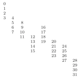
The edgeless graph for a given graph is obtained by re-moving all its edges, keeping all its nodes at the same positions. In Fig. 2, the edgeless IOG for n = 5 is de-picted.

0 1 2 3 4

5 8

6 9 16

7 10 17 11 12 18

13 19 20 14 21 24 15 22 25 23 26

27 28 29 30 31

Figure 2: The edgeless intrinsic order graph forn= 5.

For further theoretical properties and practical applica-tions of the intrinsic order and the IOG, we refer the reader to [2, 6, 7, 8].

3

Bisecting the Intrinsic Order Graph

A bisection of a graph is a partition of its vertex set into two (disjoint) subsets with half the vertices each. So, Theorem 2.3 suggests us a natural bisection of the (edgeless) graphI_ninto its two isomorphic (edgeless) sub-graphsI_n−1 and 2n−1+I_n−1.

halves, and the same happens with each one of them, and so on. In other words, the posetI_n has the self-similarity property. Figs. 1 and 2 illustrate this fact.

Let us set an adequate notation for this iterative bisection process. For alln ≥1, for all 1 ≤k ≤n, and for allk fixed binary digits ¯u₁, . . . ,u¯_k ∈ {0,1}, from now on we denote by Iu¯1,...,uk¯

n the subset of binary n-tuples whose k first (or left-most) components are constant, namely

u1= ¯u1, . . . , uk= ¯uk; while then−klast (or right-most)

components, u_k+1, . . . , u_n, take all possible values (0 or 1). More precisely,Iu¯1,...,uk¯

n is the set

(¯u₁, . . . ,u¯_k, u_k+1, . . . , u_n) (u_k+1, . . . , u_n)∈ {0,1}n−k

≡(¯u₁, . . . ,u¯_k,0, . . . ,0)₍₁₀,(¯u₁, . . . ,u¯_k,1, . . . ,1)₍₁₀

(3.1) and, obviously, the cardinality of this subposet is

_Iu¯1,...,uk¯

n ={0,1}n−k= 2n−k. (3.2)

Note that Iu¯1,...,uk¯

n can be graphically obtained after k

successive bisections ofI_n (1≤k≤n) simply by chang-ing, from right to left, the “0” and “1” bits of the vector (¯u₁, . . . ,u¯_k), by the words “first half” and “second half”, respectively.

Example 3.1 Forn= 5,k= 3 and for the upper indices (¯u₁,u¯₂,u¯₃) = (1,1,0), using (3.1), we get the subgraph

I1,1,0 5 =

(1,1,0, u₄, u₅) (u₄, u₅)∈ {0,1}2

≡(1,1,0,0,0)₍₁₀,(1,1,0,1,1)₍₁₀

= [24,27] ={24,25,26,27}

and looking at Fig. 2, we confirm that the subposet

I₅1,1,0 = [24,27] is exactly the first half (¯u₃ = 0) of the second half (¯u₂ = 1) of the second half (¯u₁ = 1) of the posetI₅. Moreover, in accordance with (3.2), we see that

I₅1,1,0 has exactly 25−3= 4 elements.

The most important property of the above bisection pro-cedure of the IOG is stated by the following Theorem.

Theorem 3.1 Letn≥1and1≤k≤n. Bisect the edge-less graph I_n into its 2k subgraphs Iu¯1,...,uk¯

n (i.e., make

k successive bisections of I_n). Replace each subgraph

Iu¯1,...,uk¯

n by an unique node labeled by its corresponding

vector of upper indices (¯u₁, . . . ,u¯_k) and weighted by its occurrence probability Pr{(¯u₁, . . . ,u¯_k)}. Then the prob-ability(weight) of each of these nodes (¯u₁, . . . ,u¯_k) coin-cides with the sum of the occurrence probabilities of all the binaryn-tuplesulying on the corresponding replaced subgraphIu¯1,...,uk¯

n . Moreover, the Hasse diagram obtained

by sorting these2k new nodes in decreasing order of their weights is precisely the IOGI_k.

Proof. First, using (3.1), we get

u∈Iu¯1,...,uk¯

n

Pr{u}

=

(uk+1,...,un)∈{0,1}n−k

Pr{(¯u₁, . . . ,u¯_k, u_k+1, . . . , u_n)}

= Pr{(¯u₁, . . . ,u¯_k)}

v∈{0,1}n−k

Pr{v}

= Pr{(¯u₁, . . . ,u¯_k)}.

Second, sorting the 2k vertices of the new con-densed graph in decreasing order of their weights Pr{(¯u₁, . . . ,u¯_k)} is equivalent to ordering the 2k binary

k-tuples (¯u₁, . . . ,u¯_k)∈ {0,1}kin decreasing order of their occurrence probabilities. Thus, the new condensed graph is, by definition, the IOGI_k.

Example 3.2 Let n= 5 and k = 2. The 2k = 22 = 4 equal-sized subgraphs obtained after k = 2 successive bisections ofI₅, are (see Fig. 2):

I₅0,0= [0,7], I₅0,1= [8,15], I₅1,0= [16,23], I₅1,1= [24,31]. Then the occurrence probability of each subgraphI¯u1,u¯2

5

(i.e., the sum of the occurrence probabilities of all the eight nodes lying on it) coincides with the occurrence probability of its corresponding binary 2-tuple (¯u₁,u¯₂). Moreover, the four subgraphs I₅0,0, I₅0,1, I₅1,0, I₅1,1 are re-placed by their corresponding binary 2-tuples (upper in-dices), (0,0) ≡ 0, (0,1) ≡ 1, (1,0) ≡ 2, (1,1) ≡ 3, and displayed –in decreasing order of their occurrence probabilities– on the digraph ofI₂(the second one from the left in Fig. 1.). So,k= 2 successive bisections ofI₅ lead toI₂, following a “nice fractal behavior”.

4

Chains in the Intrinsic Order Graph

Two elementsu, v of a poset (P,≤) are said to be com-parable if either u≤v or v ≤u. A chain in a poset is a totally ordered subset, i.e., a subset of pairwise com-parable elements. A chain u=u1 > u2 >· · ·> ul =v fromuto v is said to have length l−1. A chain is said to be saturated when no further elements can be interpo-lated between its elements. In other words, all successive relations in a saturated chain are coverings [9].

In particular, a saturated chain of length l −1 in our posetI_nis a subset u1, u2, . . . , ulof{0,1}n, such that

u1 _u2_{· · · u}l_{, i.e., u}1 _u2 _{· · · u}l _{with no other}

elements between them.

a chain decomposition into saturated chains, i.e., a set of disjoint saturated chains covering all elements ofP. Let us mention that one can define many different chain covers ofI_n. The most intuitively natural way for par-titioningI_n into saturated chains is clearly suggested by Figs. 1 or 2. Just consider the 2n−2 “columns” obtained aftern−2 successive bisections ofI_n, containing four con-secutive numbers beginning with a multiple 4kof 4, each. For instance, see the 23= 8 “columns” inI₅, depicted in Fig. 2. Next Corollary formalizes this chain cover.

Corollary 4.1 For all n≥ 2 the poset I_n can be parti-tioned into the following 2n−2 saturated chains of length

3, that we call “congruence chains(mod 4)”:

4k 4k+ 14k+ 24k+ 3 0≤k≤2n−2−1.

Proof. Clearly, for all k∈0,2n−2−1, that is, for all

k≡(u₁, . . . , u_n−2)∈ {0,1}n−2, the matrices

M4k

4k+1 =

u1 . . . un−2 0 0

u1 . . . un−2 0 1

,

M4k+1 4k+2 =

u1 . . . un−2 0 1

u1 . . . un−2 1 0

,

M4k+2 4k+3 =

u1 . . . un−2 1 0

u1 . . . un−2 1 1

have either the pattern (2.3) or the pattern (2.4). Finally, since all these saturated chains are pairwise disjoint, and they completely coverI_n, i.e.,

0≤k≤2n−2₋₁

{4k,4k+ 1,4k+ 2,4k+ 3}= [0,2n−1],

the proof is concluded.

The rest of this section is devoted to present a second chain cover of the posetI_n, far less intuitive than the con-gruence chains (mod. 4), but more relevant to the analysis of CSBSs. Basically, we shall use “diagonals” instead of “columns”, for partitioningI_n.

Lemma 4.1 (A symmetry property) For all n≥ 2, the complementary set Cc of a saturated chain C of I_n is also a saturated chain, and the elements ofCc are the complementary of the elements ofCin reverse order, i.e.,

u1 _u2_{· · · u}l _{⇔ u}lc_{· · ·u}2c_u1c_.

Proof. Clearly, the 0₀, 1₁, 0₁ and 1₀ columns in

Mu

v, respectively become

₁ 1

, 0₀, 0₁ and 1₀ columns in M_uvcc. Hence, using Theorem 2.2, we have that u v

iff M_vu has either the pattern (2.3) or the pattern (2.4) iff M_uvcc respectively has either the pattern (2.3) or the

pattern (2.4) iffvc uc.

Next theorem establishes the chain cover of the posetI_n into “diagonal” saturated chains.

Theorem 4.1 For all n ≥ 3 the poset I_n can be parti-tioned into the “diagonal” saturated chains displayed from top to bottom(and also from right to left)in its IOG.

Proof. We classify the set of “diagonal” saturated chains for coveringI_n into the following three kinds (see Defini-tion 2.1-(iii)&(iv) for the notaDefini-tion and nomenclature): (i) The chain containing alln-tuples of weights 0 and 1. This is the right-most (and also the top-most) “diagonal” chain in the digraph ofI_n:

0[1]_n= 1[2]_n= 2[3]_n = 22· · ·[n]_n = 2n−1. (4.1)

Indeed, 01, and 2i2i+1 (0≤i≤n−2) because

M0₀,...,_,...,0₀,_,0₁ and M0₀,...,_,...,0₀,_,0₁,_,1₀,_,0₀,...,_,...,0₀ have the pattern (2.3) and (2.4), respectively. (ii) The chains containing the followingn-tuples:

⎧ ⎨ ⎩

Ifnis odd: alln-tuples of weights 2,3, . . . ,n−₂1. Ifnis even:

alln-tuples of weights 2,3, . . . ,n₂ −1, thosen-tuples of weight n₂ s.t. u_n= 1.

(4.2) The construction of such chains must be performed as follows. For each fixed admissible Hamming weight m, consider all the admissible n-tuples with weightm, and sort them by lexicographic order of the vectors of posi-tions of their 1-bits. Then, beginning with the first vector [1,2, . . . , m]_n of this sorted list and ending with its last vector [n−m+ 1, n−m+ 2, . . . , n]_n, we proceed as fol-lows. Two any consecutive elementsu= [i₁, i₂, . . . , i_m]_n andv = [j₁, j₂, . . . , j_m]_n of this list (i.e., uimmediately precedesv in the list) will be consecutiven-tuples in the same saturated chain (i.e.,u v) iff their vectors of posi-tions of 1s only differ in one component (position). Oth-erwise,v will be the first element of a new chain, and we proceed exactly in the same way withvand its immediate successorwin the sorted list, and so on.

Indeed, note that, for every fixed weightm, if the vectors

u= [i₁, i₂, . . . , i_m]_n and v = [j₁, j₂, . . . , j_m]_n only differ in one component, sayi_p = j_p, then j_p =i_p+ 1. This is becausev immediately succeeds touin the list of the vectors of positions of 1s arranged by lexicographic order. But to say that the vectors ofuand v only differ in the

p-th component withj_p =i_p+ 1 is equivalent to saying that matrixM_vuhas the pattern (2.4), and thus u v. (iii) Complementary chains of those obtained in (i) & (ii): CallS the set of all binaryn-tuples included in all chains generated in steps (i) & (ii). Clearly, there are_mnbinary

n-tuples with weightm. Hence, from (4.1) and (4.2), we have that the cardinality ofS is given by

Ifnis odd: n₀+n₁+· · ·+nn−3 2

+nn−1 2

= 2n−1, Ifnis even: n₀+n₁+· · ·+nn

2−1

+1₂nn

2

so that, in both cases (n odd, neven), we have used in steps (i) & (ii) exactly half of the set {0,1}n of binary

n-tuples (whose cardinality is 2n).

Now, taking into account again (4.1) and (4.2), we have that all then-tuples of S have weight m < n₂ (with the only exception of those n-tuples of weight m = n₂ s.t.

un = 1, if n is even). Note that the complementary n

-tuple of a binaryn-tuple of weightmobviously has weight

n−m. Then all the complementary n-tuples of the n -tuples ofShave weightn−m > n−n₂ =n₂ (with the only exception of thosen-tuples of weightn−m=n−n₂ =n₂ s.t. u_n= 0, ifnis even). This implies that

S∩Sc_=∅

and this empty intersection means that, among the 2n−1 nodes ofS (i.e., the ones used in steps (i) & (ii)), there is no pair of complementaryn-tuples. Consequently, using Lemma 4.1, we conclude that it suffices to take the com-plementary chains of those covering the halfSofI_n(steps (i) & (ii)), to cover the other halfScofI_n (step (iii)). Fi-nally, since all the chains generated in this way are, by construction, saturated, pairwise disjoint, and they com-pletely cover our posetI_n, the proof is concluded.

Example 4.1 The “diagonal” chain cover ofI₄ (n= 4, even) has the following 4 chains, displayed from top to bottom (and also from right to left) inI₄ (see the right-most graph in Fig. 1, and use (2.1) for step(iii)):

(i)C₁ = ˘0[1]₄[2]₄[3]₄[4]₄¯={01248}, (ii)_C2 = ˘[1_,2]₄[1_,3]₄[1_,4]₄¯=_{359_},

(iii)C₂c = {61012},

Cc

1 = {711131415}.

Example 4.2 The “diagonal” chain cover ofI₅ (n= 5, odd) has the following 8 chains, displayed from top to bottom (and also from right to left) inI₅(see Fig. 2, and use (2.1) for step(iii)):

(i)_C1 = ˘0[1]₅[2]₅[3]₅[4]₅[5]₅¯ = {0124816},

(ii)C₂ = ˘[1,2]₅[1,3]₅[1,4]₅[1,5]₅¯={35917},

C3 = ˘[2,3]₅[2,4]₅[2,5]₅¯={61018},

C4 = ˘[3_,4]₅[3_,5]₅[4_,5]₅¯=_{122024_}, (iii)C₄c = {71119},

Cc

3 = {132125},

Cc

2 = {14222628},

Cc

1 = {152327293031}.

5

Concluding Remarks

We have partitioned the IOG for CSBSs in two different ways. The first one consists of successively bisectingI_n into smaller and smaller subgraphs. The main interest of this iterative bisection process is the following. The (ordering between the) occurrence probabilities of the 2k equal-sized subgraphs –obtained afterksuccessive bisec-tions ofI_n– exactly coincides with the (ordering between

the) occurrence probabilities of the corresponding 2k bi-naryk-tuples whose components are thek left-most bits of all nodes lying on those subgraphs. Hence,ksuccessive bisections ofI_nlead toI_k: a useful, nice, fractal property for the analysis of CSBSs! The second one consists of cov-eringI_nwith the “diagonal” chains displayed from top to bottom in its IOG. The main interest of this chain cover is the following. One of the main problems in Reliability Engineering and Risk Analysis is to determine the system elementary states with the largest occurrence probabili-ties [1]. Such elementary states are usually those hav-ing the smallest Hammhav-ing weights, and with their 1-bits placed among the right-most positions. But, precisely, the up-most “diagonal” chains of our chain partition con-tains the binaryn-tuples satisfying both conditions. This can be also applied, in Fault Tree Analysis, for evaluating the system unavailability.

References

[1] Andrews, J., Moss, B.,Reliability and Risk Assess-ment, 2nd Edition, Professional Engineering Pub-lishing, 2002.

[2] Galv´an, B, Gonz´alez, L., “Quantitative analysis of large fault trees using intrinsic ordering and the Pas-cal triangle,” Reliab Eng Syst Safety, to be pub-lished.

[3] Gonz´alez, L., “A New Method for Ordering Binary States Probabilities in Reliability and Risk Analy-sis,” Lect Notes Comp Sc, V2329, N1, pp. 137-146, 2002.

[4] Gonz´alez, L., “N-tuples of 0s and 1s: Necessary and Sufficient Conditions for Intrinsic Order,”Lect Notes Comp Sc, V2667, N1, pp. 937-946, 2003.

[5] Gonz´alez, L., “A Picture for Complex Stochastic Boolean Systems: The Intrinsic Order Graph,”Lect Notes Comput Sc, V3993, N3, pp. 305-312, 2006. [6] Gonz´alez, L., “Algorithm comparing binary string

probabilities in complex stochastic Boolean systems using intrinsic order graph,”Adv Complex Syst, V10, N1, pp. 111-143, 2007.

[7] Gonz´alez, L., “Ranking intervals in complex stochas-tic Boolean systems using intrinsic ordering,” in Ma-chine Learning and Systems Engineering, Rieger, B. B., Amouzegar, M. A., Ao, S.-I., Eds., Springer, to be published.

[8] Gonz´alez, L., Garc´ıa, D., Galv´an, B., “An Intrinsic Order Criterion to Evaluate Large, Complex Fault Trees,” IEEE Trans Reliab, V53, N3, pp. 297-305, 2004.